# code for loading the format for the notebook
import os

# path : store the current path to convert back to it later
path = os.getcwd()
os.chdir(os.path.join('..', '..', 'notebook_format'))

from formats import load_style
load_style(plot_style = False)
os.chdir(path)
# 1. magic for inline plot
# 2. magic to print version
# 3. magic so that the notebook will reload external python modules
# 4. magic to enable retina (high resolution) plots
# https://gist.github.com/minrk/3301035
%matplotlib inline
%load_ext watermark
%load_ext autoreload
%autoreload 2
%config InlineBackend.figure_format = 'retina'

import numpy as np
import pandas as pd
import seaborn as sns
import matplotlib.pyplot as plt
from datetime import datetime

%watermark -a 'Ethen' -d -t -v -p numpy,pandas,seaborn,matplotlib
Cohort Analysis
What is Cohort Analysis? and why is it valuable? To begin with, a cohort is a group of users who share something in common, be it their sign-up date, first purchase month, birth date, acquisition channel, etc. Cohort analysis is the method by which these groups are tracked over time, helping you spot trends, understand repeat behaviors (purchases, engagement, amount spent, etc.) and monitor your customer and revenue retention.
It's common for cohorts to be created based on a customer's first usage of the platform, where "usage" is dependent on your business's key metrics. For Uber or Lyft, usage would be booking a trip through one of their apps. For GrubHub, it's ordering some food. For AirBnB, it's booking a stay. With these companies, a purchase is at their core, be it taking a trip or ordering dinner — their revenues are tied to their users' purchase behavior. In others, a purchase is not central to the business model and the business is more interested in "engagement" with the platform. Facebook and Twitter are examples of this - are you visiting their sites every day? Are you performing some action on them - maybe a "like" on Facebook or a "favorite" on a tweet? Thus when building up a cohort analysis, it's important to consider the relationship between the event or interaction you're tracking and its relationship to your business model.
Example of Monthly Cohort
Imagine we have the following dataset that has the standard purchase data with IDs for the order and user, order data and purchase amount. To create our monthly cohort, we'll first have to:
- Convert our date to a monthly-time basis.
- Determine the user's cohort group based on their first order, which is the year and month in which the user's first purchase occurred.
df = pd.read_csv('relay-foods.csv')
df.head()
def parse_dmy(s):
    """
    convert string to datetime format

    References
    ----------
    http://chimera.labs.oreilly.com/books/1230000000393/ch03.html#_discussion_55
    """
    month, day, year = s.split('/')
    return datetime(int('20' + year), int(month), int(day))


# remove the $ sign from the TotalCharges column
# and convert it to float
df['TotalCharges'] = (df['TotalCharges'].
                      apply(lambda x: x.replace('$', '')).
                      astype('float'))

# strip out the year and month into a new column
df['OrderDate'] = df['OrderDate'].apply(parse_dmy)
df['OrderPeriod'] = df['OrderDate'].apply(lambda x: x.strftime('%Y-%m'))
df.head()
# convert each user id into their cohort group
df = df.set_index('UserId')
df['CohortGroup'] = (df.
                     groupby(level = 0)['OrderDate'].min().
                     apply(lambda x: x.strftime('%Y-%m')))
df = df.reset_index()
df.head()
Since we're looking at monthly cohorts, we need to aggregate users, orders, and amount spent by the CohortGroup within each month (OrderPeriod). After that, we wish to look at how each cohort has behaved in the months following their first purchase, so we'll need to index each cohort with respect to their first purchase month. For example, CohortPeriod = 1 will be the cohort's first month, CohortPeriod = 2 is their second, and so on. This allows us to compare cohorts across various stages of their lifetime.
grouped = df.groupby(['CohortGroup', 'OrderPeriod'])

# count the unique users, orders, and total revenue per Group + Period
cohorts = grouped.agg({'UserId': pd.Series.nunique,
                       'OrderId': pd.Series.nunique,
                       'TotalCharges': np.sum})

# make the column names more meaningful
renaming = {'UserId': 'TotalUsers', 'OrderId': 'TotalOrders'}
cohorts = cohorts.rename(columns = renaming)
cohorts.head()
def cohort_period(df):
    """
    Creates a `CohortPeriod` column,
    which is the Nth period based on the user's first purchase.
    """
    df['CohortPeriod'] = np.arange(len(df)) + 1
    return df


cohorts = cohorts.groupby(level = 'CohortGroup').apply(cohort_period)
cohorts.head()
We're now half way done, before we proceed on with the process, we will do some sanity checking to make sure that we did everything right by performing some simple testing. We'll test data points from the original DataFrame with their corresponding values in the new cohorts DataFrame to make sure all our data transformations worked as expected. As long as none of these raise an exception, we're good.
# unit test code chunk
mask = (df['CohortGroup'] == '2009-01') & (df['OrderPeriod'] == '2009-01')
x = df[mask]
y = cohorts.loc[('2009-01', '2009-01')]

assert np.allclose(x['UserId'].nunique(), y['TotalUsers'])
assert np.allclose(x['TotalCharges'].sum(), y['TotalCharges'])
assert np.allclose(x['OrderId'].nunique(), y['TotalOrders'])
To calculate the user retention by cohort group, We want to look at the percentage change of each CohortGroup over time -- not the absolute change. To do this, we'll first need to create a pandas Series containing each CohortGroup and its size.
# convert the CohortPeriod as indices instead of OrderPeriod
cohorts = cohorts.reset_index()
cohorts = cohorts.set_index(['CohortGroup', 'CohortPeriod'])
cohorts.head()
# create a Series holding the total size of each CohortGroup
cohorts_size = cohorts['TotalUsers'].groupby(level = 'CohortGroup').first()
cohorts_size.head()
Now, we'll need to divide the TotalUsers values in cohorts by cohort_size. Since DataFrame operations are performed based on the indices of the objects, we'll use unstack on our cohorts DataFrame to create a matrix where each column represents a CohortGroup and each row is the CohortPeriod corresponding to that group.
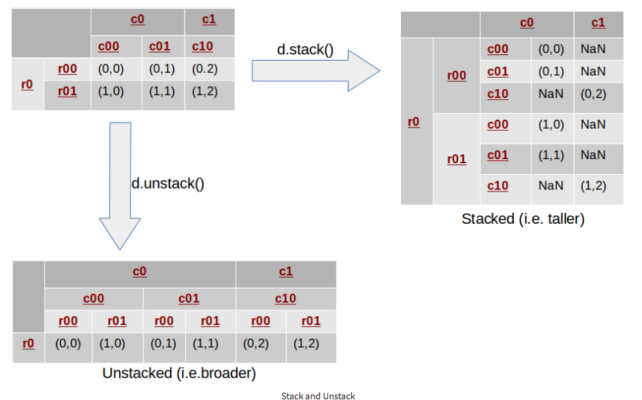
Stack/Unstack
In case you're not familiar with what unstack and stack does:
Stacking a DataFrame means moving (also rotating or pivoting) the innermost column index to become the innermost row index. The inverse operation is called unstacking. It means moving the innermost row index to become the innermost column index. The following diagram depicts the operations:
# applying it
user_retention = (cohorts['TotalUsers'].
                  unstack('CohortGroup').
                  divide(cohorts_size, axis = 1))
user_retention.head()
The resulting DataFrame, user_retention, contains the percentage of users from the cohort purchasing within the given period. For instance, 38.4% of users in the 2009-03 cohort purchased again in month 3 (which would be May 2009).
Finally, we can plot the cohorts over time in an effort to spot behavioral differences or similarities. Two common cohort charts are line graphs and heatmaps, both of which are shown below.
# change default figure and font size
plt.rcParams['figure.figsize'] = 10, 8
plt.rcParams['font.size'] = 12


user_retention[['2009-06', '2009-07', '2009-08']].plot()
plt.title('Cohorts: User Retention')
plt.xticks(range(1, 13))
plt.xlim(1, 12)
plt.ylabel('% of Cohort Purchasing')
plt.show()

Notice that the first period of each cohort is always 100% -- this is because our cohorts are based on each user's first purchase. Meaning everyone in the cohort should have made a purchase in the first month.
sns.set(style = 'white')

plt.figure(figsize = (12, 8))
plt.title('Cohorts: User Retention')
sns.heatmap(user_retention.T,
            cmap = plt.cm.Blues,
            mask = user_retention.T.isnull(),  # data will not be shown where it's True
            annot = True,  # annotate the text on top
            fmt = '.0%')  # string formatting when annot is True
plt.show()

Unsurprisingly, we can see from the above chart that fewer users tend to purchase as time goes on. However, we can also see that the 2009-01 cohort is the strongest, which enables us to ask targeted questions about this cohort compared to others -- What other attributes (besides first purchase month) do these users share which might be causing them to stick around? How were the majority of these users acquired? Was there a specific marketing campaign that brought them in? Did they take advantage of a promotion at sign-up? The answers to these questions would inform future marketing and product efforts.
Further Work
User retention is only one way of using cohorts to look at your business — we could have also looked at revenue retention. That is, the percentage of each cohort’s first month revenue returning in subsequent periods. User retention is important, but we shouldn’t lose sight of the revenue each cohort is bringing in (and how much of it is returning).
To sum it up, cohort analysis can be valuable when it comes to understanding your business's health and "stickiness" - the loyalty of your customers. Stickiness is critical since it’s far cheaper and easier to keep a current customer than to acquire a new one. For startups, it’s also a key indicator of product-market fit.
Additionally, your product evolves over time. New features are added and removed, the design changes, etc. Observing individual groups over time is a starting point to understanding how these changes affect user behavior. It’s also a good way to visualize your user retention/churn as well as formulating a basic understanding of their lifetime value.