# code for loading the format for the notebook
import os

# path : store the current path to convert back to it later
path = os.getcwd()
os.chdir(os.path.join('..',  'notebook_format'))

from formats import load_style
load_style(plot_style=False)
os.chdir(path)

# 1. magic for inline plot
# 2. magic to print version
# 3. magic so that the notebook will reload external python modules
# 4. magic to enable retina (high resolution) plots
# https://gist.github.com/minrk/3301035
%matplotlib inline
%load_ext watermark
%load_ext autoreload
%autoreload 2
%config InlineBackend.figure_format='retina'

import xgboost as xgb
import sklearn.datasets
import sklearn.metrics as metrics
from ray import tune
from sklearn.model_selection import train_test_split
from ray.tune.integration.xgboost import TuneReportCallback

%watermark -a 'Ethen' -u -d -v -iv
HyperParameter Tuning Ray Tune and HyperBand
One of steps in training a machine learning model involves hyperparameter tuning, and two most common hyper parameter tuning strategies that we might first come across are grid and random search.
In this article, we will take a look at how we can perform hyperparameter tuning using Ray Tune, as well as explore another hyperparameter tuning strategy called HyperBand.
We'll be using xgboost library as well as a sample dataset provided by scikit-learn in this example, there will be no feature preprocessing as that is not the focus of this post.
bunch = sklearn.datasets.load_breast_cancer(return_X_y=False)
print(f'number of rows: {bunch.data.shape[0]}, cols: {bunch.data.shape[1]}')
bunch.data
X_train, X_test, y_train, y_test = train_test_split(bunch.data, bunch.target, test_size=0.25)
We first train a model using the default parameters to get a baseline performance number.
model_xgb = xgb.XGBClassifier()

eval_set = [(X_train, y_train), (X_test, y_test)]
model_xgb.fit(X_train, y_train, eval_set=eval_set, verbose=10)
Hyperparameter Tuning
To use hyperparameter tuning with ray, we need to:
- Have a config dictionary, so tune can choose from a range of valid options.
- Use the config dictionary in our model object.
- Once we are done training the model, report all the necessary metrics.
config = {
    #"n_estimators": tune.randint(30, 100),
    "max_depth": tune.randint(2, 6),
    "colsample_bytree": tune.uniform(0.8, 1.0),
    "subsample": tune.uniform(0.8, 1.0),
    "learning_rate": tune.loguniform(1e-4, 1e-1)
}


def ray_train(config, X_train, y_train, X_test, y_test):
    model = xgb.XGBClassifier(**config)
    eval_set = [(X_train, y_train), (X_test, y_test)]
    model.fit(X_train, y_train, eval_set=eval_set, verbose=False)

    log_loss_test = metrics.log_loss(y_test, model.predict_proba(X_test)[:, 1])
    tune_report_metrics = {'validation_1-logloss': round(log_loss_test, 3)}
    tune.report(**tune_report_metrics)
For running hyperparameter tuning:
- We pass our training function/callable,
ray_train, as the first parameter. Here we leveragewith_parametersso we can broadcast large objects to our trainable. - We specify additional necessary arguments such as what metrics to optimize for as well as resources, and the hyperparameter tuning config space.
- ray allows us to specify a time budget along with
num_samplesof -1, this allows us to train for an infinite sample of configurations until a time budget is met.
def ray_hyperparameter_tuning(config, time_budget_s: int):
    analysis = tune.run(
        tune.with_parameters(ray_train, X_train=X_train, y_train=y_train, X_test=X_test, y_test=y_test),
        config=config,
        metric='validation_1-logloss',
        mode='min',
        num_samples=-1,
        resources_per_trial={'cpu': 8},
        time_budget_s=time_budget_s,
        verbose=1
    )
    return analysis
analysis = ray_hyperparameter_tuning(config, time_budget_s=120)
num_done_experiments = analysis.results_df[analysis.results_df['done'] == True].shape[0]

print(f'ran {num_done_experiments} hyperparameter tuning experiments')
print('best metric: ', analysis.best_result['validation_1-logloss'])
print('best config: ', analysis.best_result['config'])
HyperParameter Tuning with HyperBand
Apart from grid or random search, ray tune offers multiple hyperparameter tuning strategies, here we will be looking at one of them called Hyperband.
Hyperband can be seen as successive halving algorithm on steriods that focuses on speeding up configuration evaluation, where configuration refers to one specific set of hypereparameters. To elaborate, successive halving works by allocating a certain amount of budget to a set of hyper parameter configurations, i.e. it runs the configuration for a few iterations to get a sense of their performance, after that it will start allocating more resources to more promising configurations, while tossing away other non-performing configurations. This process repeats until one configuration remains. One of the potential drawback with successive halving is that given some finite budget $B$ (e.g. training time), and number of configurations $n$, it is not clear a priori whether we should either consider many configurations (large $n$), each with a small average training time, or the opposite, i.e. consider a small number of configurations (large $B / n$), each having a larger average training time. In other words, as practitioners, how do we decide whether we want more "depth" or more "breadth". Let's now take a look at how Hyperband aims to address this issue:
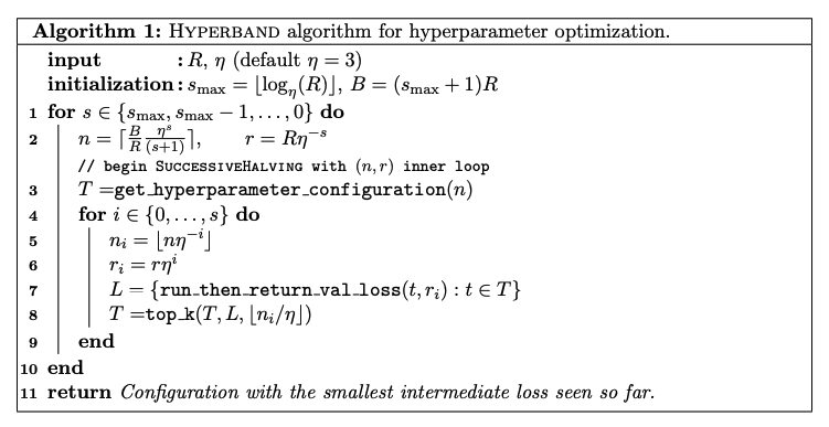
Looking at the psuedocode above, Hyperband takes in two inputs:
- R: The maximum resources that can be allocated to a single configuration, e.g. number of iterations to run the algorithm.
- $\eta$: Controls the proportion of configurations to be discarded for each round of successive halving.
Then it essentially performs a grid search over different possible values of $n$, associated with $n$ is a minimum resource $r$ that is allocated to each configuration. Lines 1-2, the outer loop, iterates over different values of $n$ and $r$, whereas the inner loop, lines 3–9, runs successive halving for the fixed $n$ and $r$.
The following code chunk provides a vanilla implementation, and returns the resource allocation table.
from random import random
from math import log, ceil
import heapq
import pandas as pd


def hyperband(R, eta):
    s_max = int(log(R) / log(eta))
    B = (s_max + 1) * R

    rows = []
    for s in reversed(range(s_max + 1)):
        # initial number of configurations
        n = int(ceil(B / R / (s + 1) * eta ** s))
        # initial number of iterations per config
        r = R * eta ** (-s)

        # get hyperparameter configurations,
        # we use a random value to represent a sampled configuration
        # from a defined hyperparameter search space
        T = [random() for _ in range(n)]
        for i in range(s + 1):
            n_configs = n * eta ** (-i)
            n_iterations = r * eta ** (i)

            # run then return validation loss, here
            # we use a random value to represent the algorithm's
            # perform after taking in n_iterations and config as inputs
            losses = [(random(), t) for t in T]

            # return top k configurations, if we are minimizing the loss
            # then we pick the top k smallest
            top_k_losses = heapq.nsmallest(int(n_configs / eta), losses)
            T = [t for loss, t in top_k_losses]

            row = [s, n_configs, n_iterations]
            rows.append(row)

    return pd.DataFrame(rows, columns=['s', 'n_configs', 'n_iterations'])
R = 81
eta = 3
hyperband(R, eta)
Notice in the last row, $s = 0$, where every configuration is allocated $R$ resources, this setting is essentially performing our good old random search. On the other extreme end of things, the first row $s = 4$, we are essentially running 81 configurations each for only 1 iteration, then proceeding on to dropping 2/3 of the bottom performing configurations. By performing a mix of more exploration and more exploitation search strategies, it automatically accomodates for scenarios where an iterative training algorithm converges very slowly and require more resources to show differentiating performance (in these scenarios, we should consider smaller $n$), as well as the opposite end of the story, where we perform aggresive early stopping to provide massive speedups and scan many different combinations.
To leverage hyperband tuning algorithm, we'll use Ray Tune's scheduler ASHAScheduler (recommended over the standard hyperband scheduler). We will also need to report our model's loss for every iteration back to tune. Ray Tune already comes with a callback class TuneReportCallback that does this without us having to implement it ourselves.
config = {
    #"n_estimators": tune.randint(30, 100),
    "max_depth": tune.randint(2, 6),
    "colsample_bytree": tune.uniform(0.8, 1.0),
    "subsample": tune.uniform(0.8, 1.0),
    "learning_rate": tune.loguniform(1e-4, 1e-1),
    "callbacks": [TuneReportCallback()]
}


def ray_train(config, X_train, y_train, X_test, y_test):
    model = xgb.XGBClassifier(**config)
    eval_set = [(X_train, y_train), (X_test, y_test)]
    model.fit(X_train, y_train, eval_set=eval_set, verbose=False)
def ray_hyperparameter_tuning(config, time_budget_s: int):
    scheduler = tune.schedulers.ASHAScheduler(
        max_t=100,
        grace_period=10,
        reduction_factor=2
    )
    analysis = tune.run(
        tune.with_parameters(ray_train, X_train=X_train, y_train=y_train, X_test=X_test, y_test=y_test),
        config=config,
        metric='validation_1-logloss',
        mode='min',
        num_samples=-1,
        scheduler=scheduler,
        resources_per_trial={'cpu': 8},
        time_budget_s=time_budget_s,
        verbose=1
    )
    return analysis
analysis = ray_hyperparameter_tuning(config, time_budget_s=120)
num_done_experiments = analysis.results_df[analysis.results_df['done'] == True].shape[0]

print(f'ran {num_done_experiments} hyperparameter tuning experiments')
print('best metric: ', analysis.best_result['validation_1-logloss'])
print('best config: ', analysis.best_result['config'])
We can retrieve the best config, and re-train our model to check if we get similar performance numbers.
best_config = analysis.best_result['config']
del best_config['callbacks']
model_xgb = xgb.XGBClassifier(**best_config)

eval_set = [(X_train, y_train), (X_test, y_test)]
model_xgb.fit(X_train, y_train, eval_set=eval_set, verbose=10)
Ray Tune provides different hyperparameter tuning algorithms other than the classic grid or random search, here we only looked at one of them, Hyperband.
Caveat: If learning rate is a hyperparameter, smaller values will likely result in inferior performance at the beginning, but may outperform other configurations if given sufficent amount of time. Hence, when using hyperhand like hyperparameter tuning methods, it might not be able to find the small learning rate and many iterations combinations that can squeeze out performance.
Reference
- Ray Documentation: Tuning XGBoost parameters
- Blog: Tuning hyperparams fast with Hyperband
- Blog: A (Slightly) Better Budget Allocation for Hyperband
- Blog: Hyper-parameter optimization algorithms: a short review
- Blog: HyperBand and BOHB: Understanding State of the Art Hyperparameter Optimization Algorithms
- Paper: L. Li, K. Jamieson, G. DeSalvo, A. Rostamizadeh, A. Talwalkar - Hyperband: A Novel Bandit-Based Approach to Hyperparameter Optimization (2016)