%load_ext watermark
%load_ext autoreload
%autoreload 2

import os
import torch
from transformers import AutoModelForCausalLM, AutoTokenizer
from llmcompressor import oneshot
from llmcompressor.modifiers.quantization import QuantizationModifier

%watermark -a 'Ethen' -d -u -v -iv
FP8 Quantization
Why Quantization
The diagram below shows the GPU memory hierarchy, simplified/adapted from [4]. Quantization helps at each level:
                    ┌──────────────────────────────────────┐
                    │           TENSOR CORES               │  ← compute AX+b
                    │  (compute units inside each SM;      │    ×N per forward pass
                    │   read operands from SRAM)           │
                    └───────────────────▲──────────────────┘
                                        │  operands
                    ┌───────────────────┴──────────────────┐
                    │           SM SRAM (on-chip)          │  ← registers, L1, shared mem
                    │  smallest, fastest                   │    one pool per SM
                    └───────────────────▲──────────────────┘
                                        │
    ════════════════════════════════════╪════════════════════════════════════
       HBM → SM bandwidth               │   ▶ every forward pass streams the
                                        │     layer weights across this link
                                        │   ▶ quantization shrinks the bytes
                                        │     that cross it
    ════════════════════════════════════╪════════════════════════════════════
                                        │
                    ┌───────────────────┴──────────────────┐
                    │           GPU HBM (off-chip DRAM)    │  ← what nvidia-smi reports
                    │  smaller than CPU RAM, but faster    │
                    │  ▶ model weights                     │
                    │  ▶ KV cache                          │
                    │  ▶ activations                       │
                    └───────────────────▲──────────────────┘
                                        │
                          PCIe / NVLink │   ×1 at model load
                                        │   (one-time cost)
                    ┌───────────────────┴──────────────────┐
                    │           CPU MAIN MEMORY (DRAM)     │
                    │  largest, slowest                    │
                    │  ▶ checkpoint loaded from disk       │
└──────────────────────────────────────┘- CPU to GPU load (one time): A smaller checkpoint loads faster. Since this happens once at startup and isn't on the hot path, it's a secondary benefit.
- HBM (High Bandwidth Memory) Capacity: BF16 uses 2 bytes per parameter, FP8 cuts that to 1 byte. Halving the weight footprint lets us serve a model using fewer GPUs, fit a larger model on the same hardware, or free up additional memory for a larger KV cache and batch size.
- HBM -> SM (Streaming Multiprocessor) bandwidth: Every forward pass streams layer weights from HBM onto the chip, so fewer bytes per weight means less data to move. This matters most at small batch sizes, where GPU spends most of its time waiting for weights rather than computing.
- Tensor cores compute: GPUs with dedicated FP8 tensor cores, such as Hopper (H100/H200/GH200) or Ada Lovelace (L40), etc. offer higher matmul throughput in FP8 than in BF16.
As the empirical results later in this notebook show, FP8 quantization delivers these gains with minimal quality loss.
FP8 Representation
Just as 96.0 = 1.5 × 64 = 1.5 × $2^6$ in scientific notation, to represent a decimal number like 96.0 using only 8 bits (eight 0s or 1s) in binary notation is comprised of three parts:
- Sign: is it positive or negative? positive
- Exponent ("how big"): which power of 2? $2^6$ = 64
- Mantissa ("where between"): where between 64 and the next power of 2 (128)? halfway (1.5×)
FP8 e4m3 format encodes exactly these three parts in 8 bits:
[S][E E E E][M M M]
1 4 3 = 8 bits total- Sign (1 bit): 0 = positive, 1 = negative
- Exponent (4 bits): Determines the magnitude/scale — which power of 2 the number lives near. 4 bits can store values 0-15, we subtract a bias of 7 to recover the actual power. For representing 96, the exponent bits are 1101 ($2^3 + 2^2 + 2^0 = 13$), producing an actual power is 13-7 = 6. This tells us our number lies in the range of $2^6$ to $2^7$
- Mantissa (3 bits): Determines precision within that range, i.e. how we can pinpoint a value between consecutive powers of 2. With 3 bits, we get $2^3 = 8$ evenly spaced positions. For 96, we need to locate where it falls between 64 and 128. Using the formula $\text{value} = 2^{\text{exponent}} \times (1 + \text{mantissa}/8)$, a mantissa of $100 = 4$ places us 4/8 of the way from 64 to 128: $64 \times (1 + 4/8) = 64 \times 1.5 = 96$.
Putting it together, 96.0 in FP8 e4m3 = 0 1101 100. If our real number is 95.0, it would get "rounded" to the closest FP8 value of 96, that's the quantization error.
E4M3 vs E5M2
Two FP8 formats exist, optimized for different roles:
┌────────┬───────┬────────┬───────┬─────────────────────────┐
│ Format │ S/E/M │ Range  │ Steps │ Typical use             │
├────────┼───────┼────────┼───────┼─────────────────────────┤
│ E4M3   │ 1/4/3 │ ±448   │ 8     │ Weights & activations   │
├────────┼───────┼────────┼───────┼─────────────────────────┤
│ E5M2   │ 1/5/2 │ ±57344 │ 4     │ Gradients               │
└────────┴───────┴────────┴───────┴─────────────────────────┘- S/E/M = sign / exponent / mantissa bits.
- Steps = number of representable values between consecutive powers of 2 (2^mantissa bits).
- E4M3 trades range for precision — better for forward pass weights/activations where values cluster in a narrower band. E5M2 trades precision for range — typically used for backward pass gradients which can spike during training.
print(torch.finfo(torch.float8_e4m3fn))
print(torch.finfo(torch.float8_e5m2))
Quantization Equation
To convert high precision tensor into lower precision ones like FP8, we apply a scaling factor to map values into representable range:
$$ X_{FP8}=\text{clip}\left(\text{round}\left(X\times S\right),-V_{max},V_{max}\right) $$Where:
- $S$ is the scaling factor.
- $V_{max}$ is the maximum representable value of lower precision FP8 format (e.g. 448 for E4M3).
- round means round to nearest representable value in the target format, not round to integer.
- clip forces any value overflowing the range back into the legal boundaries.
To dequantize back to high precision during computation, we multiply by the inverse:
$$ X_{high\_res}=X_{FP8}\times \frac{1}{S} $$Choose Scaling Strategy
Because FP8 has a narrower dynamic range, picking the right scaling factor $S$ is critical to avoid severe accuracy loss. Two primary strategies are used:
Static Scaling
- How: Pre-calculate a fixed scale factor using calibration dataset before deployment.
- Pros: Zero runtime overhead.
- Cons: Accuracy degrades if real-world data drifts from calibration data.
- Typically used for weights as they don't change after loading.
Dynamic Scaling
- How: Calculate tensor's maximum absolute value, $max(|X|)$ on the fly during runtime, and compute scaling value via $S = \frac{V_{max}}{\text{max}(\vert{}X\vert{})}$
- Pros: Maximizes accuracy regardless of input distribution.
- Cons: Introduces a minor hardware overhead to find the maximum value.
- Typically used for activations where distribution changes every forward pass based on input.
# Example tensor in bf16
tensor = torch.randn(4, 4, dtype=torch.bfloat16)

# Quantize: X_FP8 = clip(round(X × S), -V_max, V_max)
V_max = 448.0
S = V_max / tensor.abs().max()

# .to(float8) handles rounding to nearest representable FP8 value
# No explicit torch.round() needed — that's carryover notation for integer type quantization
tensor_fp8 = (tensor * S).clamp(-V_max, V_max).to(torch.float8_e4m3fn)

# Dequantize
tensor_restored = tensor_fp8.to(torch.bfloat16) / S

# Check error
print(f"Original:\n{tensor}")
print(f"fp8:\n{tensor_fp8}")
print(f"Restored:\n{tensor_restored}")

def relative_error(approx, ref):
    """A relative Frobenius-norm error measures the difference between a true tensor and its approximation,
    scaled by the magnitude of the true tensor.
    """
    return (approx - ref).float().norm() / ref.float().norm()

print(f"original vs restored error:  {relative_error(tensor, tensor_restored):.6f}")
How FP8 Matmul Works at the Hardware Level
The speedup comes from H100/H200 tensor cores that natively multiply FP8 operands:
Input A (FP8) × Input B (FP8) → Accumulate in FP32 → Output (BF16 or FP8)
Both inputs are stored and loaded in FP8 (half the memory bandwidth), the multiply-accumulate runs in FP32 to prevent rounding errors from compounding across dot products, finally the output is cast back to a desired output type.
A_bf16 = torch.randn(128, 4096, dtype=torch.bfloat16, device="cuda")
B_bf16 = torch.randn(512, 4096, dtype=torch.bfloat16, device="cuda")

# ── Ground truth: full bf16 matmul ──
C_bf16 = A_bf16 @ B_bf16.T
C_bf16
# ── FP8 matmul with FP32 accumulation (what H100 tensor cores do) ──
# Step 1: Quantize both operands to FP8
V_max = 448.0

scale_A = V_max / A_bf16.abs().max()
scale_B = V_max / B_bf16.abs().max()

A_fp8 = (A_bf16 * scale_A).clamp(-V_max, V_max).to(torch.float8_e4m3fn)
B_fp8 = (B_bf16 * scale_B).clamp(-V_max, V_max).to(torch.float8_e4m3fn)

# Step 2: Matmul — upcast to FP32 for the multiply-accumulate
# (On real H100 hardware, this happens inside the tensor core automatically.
#  Here we simulate it explicitly since torch.matmul doesn't support FP8 directly.)
C_fp8_accum32 = (A_fp8.to(torch.float32) @ B_fp8.T.to(torch.float32))

# Step 3: Undo the scaling and cast output to bf16
C_fp8_accum32 = (C_fp8_accum32 / (scale_A * scale_B)).to(torch.bfloat16)
print(C_fp8_accum32)
We can also perform a parity check with pytorch native _scaled_mm method, which is one of the method vllm uses if other hardware specialized kernels aren't available.
C_hardware = torch._scaled_mm(
    A_fp8, # [M, K] row major
    B_fp8.T, # [K, N] column major
    # scale should be float32
    scale_a=(1.0 / scale_A).to(torch.float32),
    scale_b=(1.0 / scale_B).to(torch.float32),
    # accumulates in FP32 internally, outputs bf16
    out_dtype=torch.bfloat16,
)
C_hardware
print(f"FP8 + FP32 accumulate vs BF16:  {relative_error(C_fp8_accum32, C_bf16):.6f}")
print(f"FP8 + FP32 accumulate vs scale mm:  {relative_error(C_fp8_accum32, C_hardware):.6f}")
Granularity
Apart from scaling strategy, we can also determine scaling granularity. i.e. how many elements share a single scale factor e.g.
Per-tensor -- one scale for the entire matrix:
Weight W [4096 x 4096]:
  scale = 448 / max(|W|)     # 1 scalar
Per-channel -- one scale per output row:
Weight W [4096 x 4096]:
  scale[i] = 448 / max(|W[i, :]|)
Per-block, e.g. [128x128] -- one scale per 128x128 tile:
Weight W [4096 x 4096]:
  For each 128x128 block:
scale[i,j] = 448 / max(|block_ij|)Implementation
We use llmcompressor to implement a FP8_DYNAMIC quantization [1]. This is a W8A8 method where:
- Weights are quantized statically per channel offline to FP8.
- Activations are scaled dynamically per token at inference time to FP8. No calibration data is used.
Layers:
As a rule of thumb for quantization, we target only Linear layers, since FP8 tensor cores main purpose is to accelerate matrix multiplications. Normalization layers and embeddings are division sensitive or comprised of elementwise/lookup operations with comparatively fewer parameters, so quantizing them offers very negligible speedup or memory savings. Among the Linear layers, we further exclude those where small numerical errors can flip discrete decisions, such as lm_head, mtp speculative head (token selection), MOE router gates (expert assignment). We also exclude linear attention layers, where errors accumulate through recurrent state.
model_name = "Qwen3-Next-80B-A3B-Instruct"
cache_dir = "/shared/data"
model_path = f"{cache_dir}/{model_name}"

# Save to disk in compressed-tensors format (vLLM compatible)
quantized_model_name = model_name.rstrip("/").split("/")[-1] + "-FP8-Dynamic"
quantized_model_path = f"{cache_dir}/{quantized_model_name}"
model = AutoModelForCausalLM.from_pretrained(model_path, cache_dir=cache_dir)
tokenizer = AutoTokenizer.from_pretrained(model_path, cache_dir=cache_dir)
recipe = QuantizationModifier(
    targets=["Linear"],
    scheme="FP8_DYNAMIC",
    ignore=[
        "lm_head",
        # moe router and shared expert gate
        "re:.*mlp.gate$",
        "re:.*mlp.shared_expert_gate$",
        # linear attention layers (GatedDeltaNet)
        "re:.*linear_attn.*",
        # mtp speculative head
        # "re:^mtp.*",
    ],
)

# Apply quantization (no calibration data needed for FP8_DYNAMIC)
oneshot(model=model, recipe=recipe)

#!du -h -d 1 $model_path
#!du -h -d 1 $quantized_model_path
model.save_pretrained(quantized_model_path, save_compressed=True)
tokenizer.save_pretrained(quantized_model_path)
We can check disk usage of the quantized checkpoint to confirm its lower size, and vllm serve this quantized checkpoint to check for performance parity as subsequent step.
To close out this document, we will take a closer look at some empirical numbers from a quantization study on Deepseek-R1 distilled models [3]
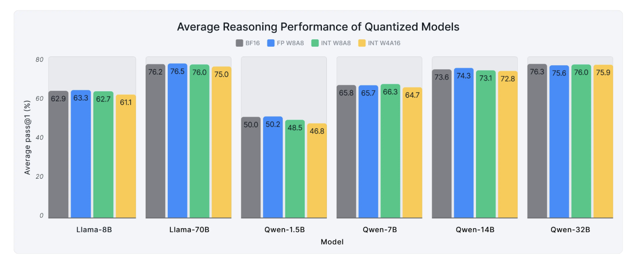
- Performance recovery: FP W8A8 is nearly lossless, matching BF16 across reasoning benchmarks. INT W8A8 closely tracks FP W8A8, making them a practical alternative for Ampere and older devices that lack dedicated FP8 tensor cores. INT W4A16 can exhibit more noticeable performance degradation, particularly on smaller models. The more aggressive 4 bit weight compression has less room for error when the model itself has fewer parameters to absorb quantization noise.
- Larger quantized model can beat a smaller unquantized one: Most quantization discussion frame the question as "how well does the quantized model recover the unquantized baseline?" But the more practical deployment decision is: should we run a smaller model at full precision or a quantized larger model. Suppose we have a setup where we can only afford a 7B full precision model, quantizing larger model opens a second pathway where we can take a 14B or 32B model quantize it down to W8 or W4 so it fits the same budget, and inherit larger model variant's stronger base capability. From the table above, we can see the quantized larger model typically wins on quality despite performance loss during compression, because model scale offers more performance gain than the last few percent of numerical precision.
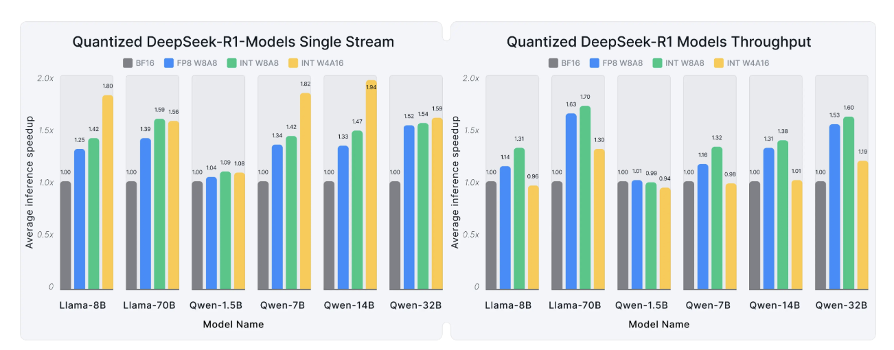
Inference speedups: The same study profiled throughput across chat, instruction following, summarization, RAG, and coding workloads on A6000, A100, and H100 GPUs:
- W8A8 wins on throughput, particularly for larger models, averaging 1.3 - 1.7x improvements across workloads. By compressing both weights and activations, memory bandwidth savings compound with faster matmuls.
- W4A16 delivers the highest speedup for single stream low latency deployments. With only 1 input in flight, the workload is memory bandwidth bound and 4 bit weights cuts the bytes moved from HBM to SM to a quarter compared to BF16.
- Smaller model like 1.5B see minimal speedup on tested GPUs. Their BF16 variant is already lightweight enough that GPU compute isn't the bottleneck, so quantization has little headroom.