# code for loading the format for the notebook
import os

# path : store the current path to convert back to it later
path = os.getcwd()
os.chdir(os.path.join('..', 'notebook_format'))

from formats import load_style
load_style(plot_style = False)
os.chdir(path)

import os
import string
import numpy as np
import pandas as pd
import matplotlib.pyplot as plt
from time import time
from collections import Counter
from keras.utils import to_categorical
from keras.utils.data_utils import get_file
from keras.models import Sequential, load_model
from keras.layers import Embedding, LSTM, Dense
from keras.callbacks import EarlyStopping, ModelCheckpoint

# 1. magic so that the notebook will reload external python modules
# 2. magic for inline plot
# 3. magic to enable retina (high resolution) plots
# https://gist.github.com/minrk/3301035
# 4. magic to print version
%load_ext autoreload
%autoreload 2
%matplotlib inline
%config InlineBackend.figure_format = 'retina'
%load_ext watermark
%watermark -a 'Ethen' -d -t -v -p keras,numpy,matplotlib,tensorflow
Keras RNN (Recurrent Neural Network) - Language Model
Language Modeling (LM) is one of the foundational task in the realm of natural language processing (NLP). At a high level, the goal is to predict the n + 1 token in a sequence given the n tokens preceding it. A well trained language model are used in applications such as machine translation, speech recognition or to be more concrete business applications such as Swiftkey.
Language Model can operate either at the word level, sub-word level or character level, each having its own unique set of benefits and challenges. In practice word-level LMs tends to perform better than character-level LMs, but suffer from increased computational cost due to large vocabulary sizes. Apart from that it also requires more data preprocessing such as dealing with infrequent words and out of vocabulary words. On the other hand, character-level LMs do not face these issues as the vocabulary only consists of a limited set of characters. This, however, is not without drawbacks. Character-level LMs is more prone to vanishing gradient problems, as given a sentence "I am happy", a word-level LM would potentially treat this as 3 time steps (3 words/tokens), while a character-level LM would treat this as 8 time steps (8 characters), hence as the number of words/tokens in a sentence increase, the time step that the character-level LM needs to capture would be substantially higher than that of a word-level LM. To sum it up in one sentence. The distinction between word-level LMs and character-level LMs suggests that achieving state-of-art result for these two tasks often requires different network architectures and are usually not readily transferable.
Implementation
This documentation demonstrates the basic workflow of:
- Preparing text for developing a word-level language model.
- Train an neural network that contains an embedding and LSTM layer then used the learned model to generate new text with similar properties as the input text.
def elapsed(sec):
    """
    Converts elapsed time into a more human readable format.

    Examples
    --------
    from time import time

    start = time()
    # do something that's worth timing, like training a model
    elapse = time() - start
    elapsed(elapse)
    """
    if sec < 60:
        return str(sec) + ' seconds'
    elif sec < (60 * 60):
        return str(sec / 60) + ' minutes'
    else:
        return str(sec / (60 * 60)) + ' hours'
path = get_file('nietzsche.txt', origin = 'https://s3.amazonaws.com/text-datasets/nietzsche.txt')
with open(path, encoding = 'utf-8') as f:
    raw_text = f.read()

print('corpus length:', len(raw_text))
print('example text:', raw_text[:150])
As with all text analysis, there are many preprocessing steps that needs to be done to make the corpus more ready for downstream modeling, here we'll stick to some really basic ones as this is not the main focus here. Steps includes:
- We will be splitting the text into words/tokens based on spaces, and from the first few words, we can see that some words are separated by "--", hence we'll replace that with a space.
- Removing punctuation marks and retain only alphabetical words.
# ideally, we would save the cleaned text, to prevent
# doing this step every single time
tokens = raw_text.replace('--', ' ').split()
cleaned_tokens = []
table = str.maketrans('', '', string.punctuation)
for word in tokens:
    word = word.translate(table)
    if word.isalpha():
        cleaned_tokens.append(word.lower())

print('sampled original text: ', tokens[:10])
print('sampled cleaned text: ', cleaned_tokens[:10])
The next step is to map each distinct word into integer so we can convert words into integers and feed them into our model later.
# build up vocabulary,
# rare words will also be considered out of vocabulary words,
# this will be represented by an unknown token
min_count = 2
unknown_token = '<unk>'
word2index = {unknown_token: 0}
index2word = [unknown_token]

filtered_words = 0
counter = Counter(cleaned_tokens)
for word, count in counter.items():
    if count >= min_count:
        index2word.append(word)
        word2index[word] = len(word2index)
    else:
        filtered_words += 1

num_classes = len(word2index)
print('vocabulary size: ', num_classes)
print('filtered words: ', filtered_words)
Recall that a language model's task is to take $n$ words and predict the $n + 1$ word, hence a key design decision is how long the input sequence should be. There is no one size fits all solution to this problem. Here, we will split them into sub-sequences with a fixed length of 40 and map the original word to indices.
# create semi-overlapping sequences of words with
# a fixed length specified by the maxlen parameter
step = 3
maxlen = 40
X = []
y = []
for i in range(0, len(cleaned_tokens) - maxlen, step):
    sentence = cleaned_tokens[i:i + maxlen]
    next_word = cleaned_tokens[i + maxlen]
    X.append([word2index.get(word, 0) for word in sentence])
    y.append(word2index.get(next_word, 0))

# keras expects the target to be in one-hot encoded format,
# ideally we would use a generator that performs this conversion
# only on the batch of data that is currently required by the model
# to be more memory-efficient
X = np.array(X)
Y = to_categorical(y, num_classes)
print('sequence dimension: ', X.shape)
print('target dimension: ', Y.shape)
print('example sequence:\n', X[0])
# define the network architecture: a embedding followed by LSTM
embedding_size = 50
lstm_size = 256
model1 = Sequential()
model1.add(Embedding(num_classes, embedding_size, input_length = maxlen))
model1.add(LSTM(lstm_size))
model1.add(Dense(num_classes, activation = 'softmax'))
model1.compile(loss = 'categorical_crossentropy', optimizer = 'adam')
print(model1.summary())
def build_model(model, address = None):
    """
    Fit the model if the model checkpoint does not exist or else
    load it from that address.
    """
    if address is not None or not os.path.isfile(address):
        stop = EarlyStopping(monitor = 'val_loss', min_delta = 0,
                             patience = 5, verbose = 1, mode = 'auto')
        save = ModelCheckpoint(address, monitor = 'val_loss',
                               verbose = 0, save_best_only = True)
        callbacks = [stop, save]

        start = time()
        history = model.fit(X, Y, batch_size = batch_size,
                            epochs = epochs, verbose = 1,
                            validation_split = validation_split,
                            callbacks = callbacks)
        elapse = time() - start
        print('elapsed time: ', elapsed(elapse))
        model_info = {'history': history, 'elapse': elapse, 'model': model}
    else:
        model = load_model(address)
        model_info = {'model': model}

    return model_info


epochs = 40
batch_size = 32
validation_split = 0.2
address1 = 'lstm_weights1.hdf5'
print('model checkpoint address: ', address1)
model_info1 = build_model(model1, address1)
In order to test the trained model, one can compare the model's predicted word against what the actual word sequence are in the dataset.
def check_prediction(model, num_predict):
    true_print_out = 'Actual words: '
    pred_print_out = 'Predicted words: '
    for i in range(num_predict):
        x = X[i]
        prediction = model.predict(x[np.newaxis, :], verbose = 0)
        index = np.argmax(prediction)
        true_print_out += index2word[y[i]] + ' '
        pred_print_out += index2word[index] + ' '

    print(true_print_out)
    print(pred_print_out)


num_predict = 10
model = model_info1['model']
check_prediction(model, num_predict)
Despite not being a perfect match, we can see that there is still a rough correspondence between the predicted token versus the actual one. To train the network which can perform better at language modeling requires a much larger corpus and more training and optimization. But, hopefully, this post has given us a basic understanding on the general process of building a language model.
The following section lists out some ideas worth trying:
- Sentence-wise model. When generating the sub-sequences for the language model, we could perform a sentence detection first by splitting the documents into sentences then pad each sentence to a fixed length (length can be determined by the longest sentence length).
- Simplify vocabulary. Perform further text preprocessing such as removing stop words or stemming.
- Hyperparameter tuning. e.g. size of embedding layer, LSTM layer, include dropout, etc. See if a different hyperparameter setting leads to a better model. Although, if we wish to build a stacked LSTM layer using keras then some changes to the code above is required, elaborated below:
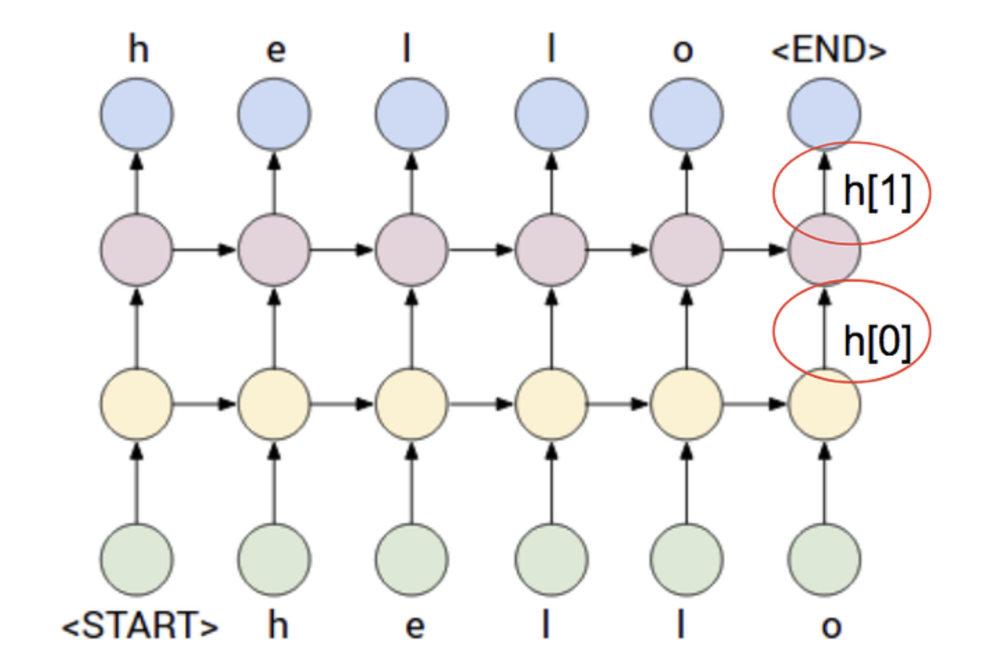
When stacking LSTM layers, rather than using the last hidden state as the output to the next layer (e.g. the Dense layer) all the hidden states will be used as an input to the subsequent LSTM layer. In other words, a stacked LSTM will have an output for every time step as oppose to 1 output across all time steps. The diagram depicts the pattern for what 2 layers would look like:
The next couple of code chunks illustrates the difference. So suppose we have two input example (batch size of 2) both having a fixed time step of 3.
from keras.models import Model
from keras.layers import Input

# using keras' functional API
seq_len = 3
n_features = 1
hidden_size = 4
data = np.array([[0.1, 0.2, 0.3], [0.15, 0.45, 0.25]]).reshape(-1, seq_len, n_features)

inputs = Input(shape = (seq_len, n_features))
lstm = LSTM(hidden_size)(inputs)
model = Model(inputs = inputs, outputs = lstm)
prediction = model.predict(data)
print('dimension: ', prediction.shape)
prediction
Looking at the output by the LSTM layer, we can see that it outputs a single (the last) hidden state for the input sequence. If we're to build a stacked LSTM layer, then we would need to access the hidden state output for each time step. This can be done by setting return_sequences argument to True when defining our LSTM layer, as shown below:
inputs = Input(shape = (seq_len, n_features))
lstm = LSTM(hidden_size, return_sequences = True)(inputs)
model = Model(inputs = inputs, outputs = lstm)

# three-dimensional output, so apart from the batch size and
# lstm hidden layer's size there's also an additional dimension
# for the number of time steps
prediction = model.predict(data)
print('dimension: ', prediction.shape)
prediction
When stacking LSTM layers, we should specify return_sequences = True so that the next LSTM layer has access to all the previous layer's hidden states.
# two-layer LSTM example, this is not trained
model2 = Sequential()
model2.add(Embedding(num_classes, embedding_size, input_length = maxlen))
model2.add(LSTM(256, return_sequences = True))
model2.add(LSTM(256))
model2.add(Dense(num_classes, activation = 'softmax'))
model2.compile(loss = 'categorical_crossentropy', optimizer = 'adam')
print(model2.summary())
Reference
- Blog: Stacked Long Short-Term Memory Networks
- Blog: Text Generation With LSTM Recurrent Neural Networks in Python with Keras
- Blog: How to Develop a Word-Level Neural Language Model and Use it to Generate Text
- Blog: Keras LSTM tutorial – How to easily build a powerful deep learning language model
- Blog: Understand the Difference Between Return Sequences and Return States for LSTMs in Keras
- Paper: S. Merity, N. Keskar, R. Socher - An Analysis of Neural Language Modeling at Multiple Scales (2018)