# code for loading the format for the notebook
import os

# path : store the current path to convert back to it later
path = os.getcwd()
os.chdir(os.path.join('..', '..', 'notebook_format'))

from formats import load_style
load_style(css_style='custom2.css', plot_style=False)
os.chdir(path)

# 1. magic for inline plot
# 2. magic to print version
# 3. magic so that the notebook will reload external python modules
# 4. magic to enable retina (high resolution) plots
# https://gist.github.com/minrk/3301035
%matplotlib inline
%load_ext watermark
%load_ext autoreload
%autoreload 2
%config InlineBackend.figure_format='retina'

import os
import math
import time
import spacy
import random
import torch
import numpy as np
import torch.nn as nn
import torch.optim as optim
from torchtext.datasets import Multi30k
from torchtext.data import Field, BucketIterator

%watermark -a 'Ethen' -d -t -v -p numpy,torch,torchtext,spacy
Seq2Seq With Attention
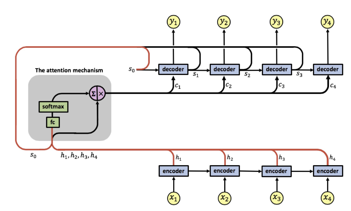
Seq2Seq framework involves a family of encoders and decoders, where the encoder encodes a source sequence into a fixed length vector from which the decoder picks up and aims to correctly generates the target sequence. The vanilla version of this type of architecture looks something along the lines of:
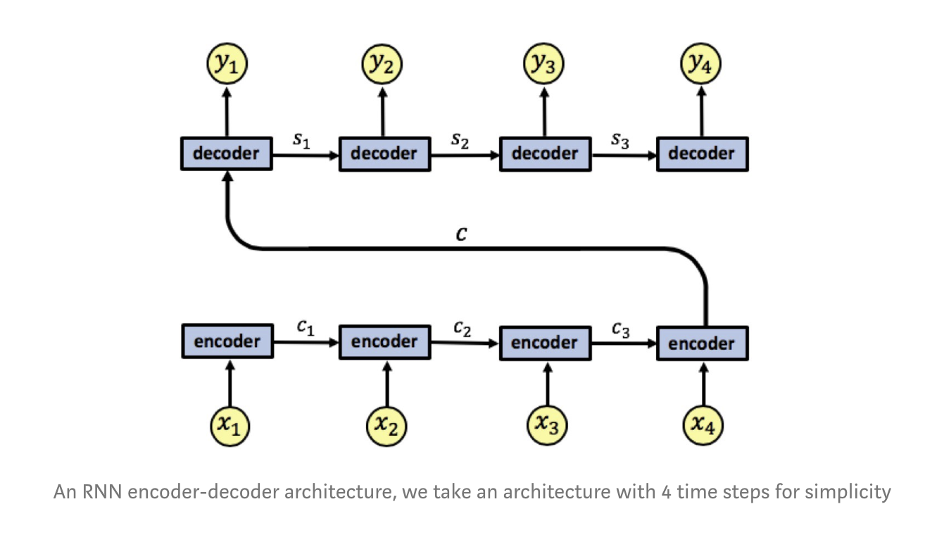
The RNN encoder has an input sequence $x_1, x_2, x_3, x_4$. We denote the encoder states by $c_1, c_2, c_3$. The encoder outputs a single output vector $c$ which is passed as input to the decoder. Like the encoder, the decoder is also a single-layered RNN, we denote the decoder states by $s_1, s_2, s_3$ and the network's output by $y_1, y_2, y_3, y_4$. A problem with this vanilla architecture lies in the fact that the decoder needs to represent the entire input sequence $x_1, x_2, x_3, x_4$ as a single vector $c$, which can cause information loss. In other words, the fixed-length context vector is hypothesized to be the bottleneck in this framework.
The attention mechanism that we'll be introducing here extends this approach by allowing the model to soft search for parts of the source sequence that are relevant to predicting the target sequence, which looks like the following:
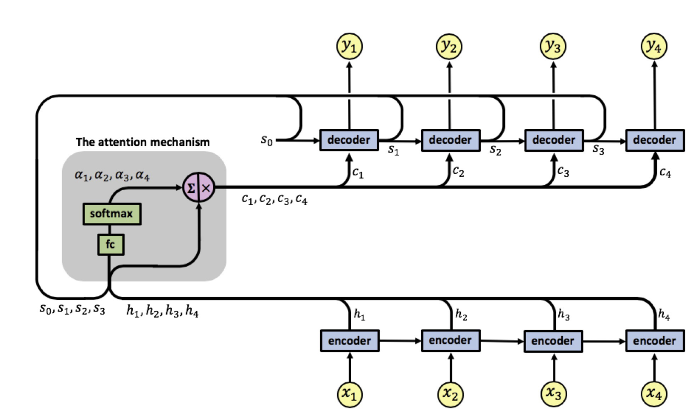
The attention mechanism is located between the encoder and the decoder, its input is composed of the encoder's output vectors $h_1, h_2, h_3, h_4$ and the states of the decoder $s_0, s_1, s_2, s_3$, the attention's output is a sequence of vectors called context vectors denoted by $c_1, c_2, c_3, c_4$.
These context vectors enable the decoder to focus on certain parts of the input when predicting its output. Each context vector is a weighted sum of the encoder's output vectors $h_1, h_2, h_3, h_4$, where each vector $h_i$ contains information about the whole input sequence with a strong focus on the parts surrounding the i-th vector of the input sequence. The vectors $h_1, h_2, h_3, h_4$ are scaled by weights $\alpha_{ij}$ capturing the degree of relevance of input $x_j$ to output at time $i$, $y_i$. The context vectors $c_1, c_2, c_3, c_4$ are calculated by:
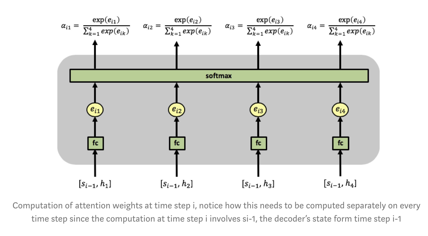
\begin{align} c_i = \sum_{j=1}^4 a_{ij} h_j \end{align}The attention weights $a_{ij}$ are learned using an additional fully-connected network, denoted by $fc$, whose input consists of the decoder's hidden state $s_0, s_1, s_2, s_3$ and the encoder's output $h_1, h_2, h_3, h_4$. It's computation can be more formally defined by:
\begin{align} a_{ij} = \frac{exp(e_{ij})}{\sum_{k=1}^4exp(e_{ik})} \end{align}Where:
\begin{align} e_{ij} = fc(s_{i-1}, h_j) \end{align}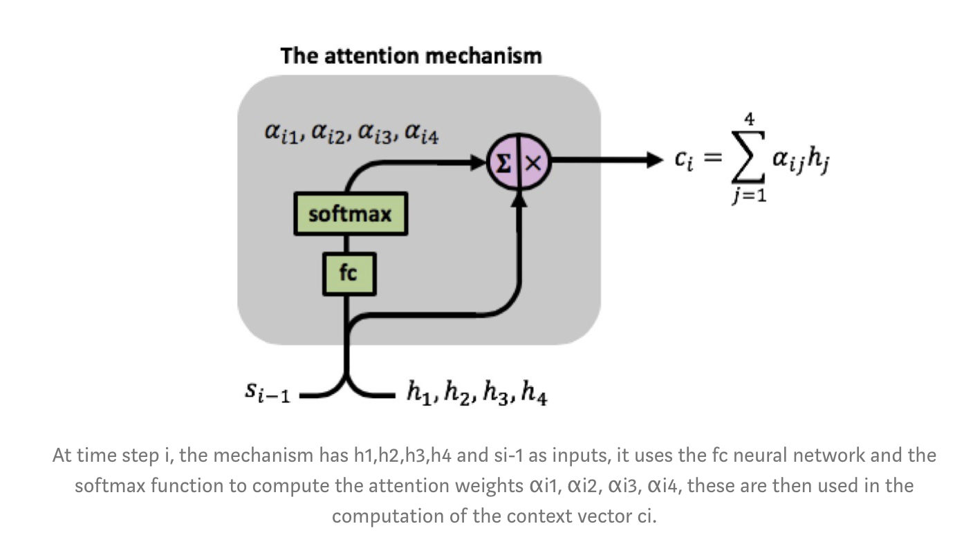
As can be seen in the above image, the fully-connected network receives the concatenation of vectors $[s_{i-1}, h_i]$ as input at time step $i$. The network has a single fully-connected layer, the outputs of the layer, denoted by $e_{ij}$, are passed through a softmax function computing the attention weights, which lie in $[0,1]$.
Note that we are using the same fully-connected network for all the concatenated pairs $[s_{i-1},h_1], [s_{i-1},h_2], [s_{i-1},h_3], [s_{i-1},h_4]$, meaning there is a single network learning the attention weights.
To re-emphasize the attention weights $\alpha_{ij}$ reflects the importance of $h_j$ with respect to the previous hidden state $s_{i−1}$ in deciding the next state $s_i$ and generating $y_i$. A large $\alpha_{ij}$ attention weight causes the RNN to focus on input $x_j$ (represented by the encoder's output $h_j$), when predicting the output $y_i$.
We can talk through an iteration of the algorithm to see how it all ties together.
The first computation performed is the computation of vectors $h_1, h_2, h_3, h_4$ by the encoder. These are then used as inputs to the attention mechanism. This is where the decoder is first involved by inputting its initial state vector $s_0$ (note that for this initial state of the decoder, we often times use the hidden state from the encoder) and we have the first attention input sequence $[s_0, h_1], [s_0, h_2], [s_0, h_3], [s_0, h_4]$.
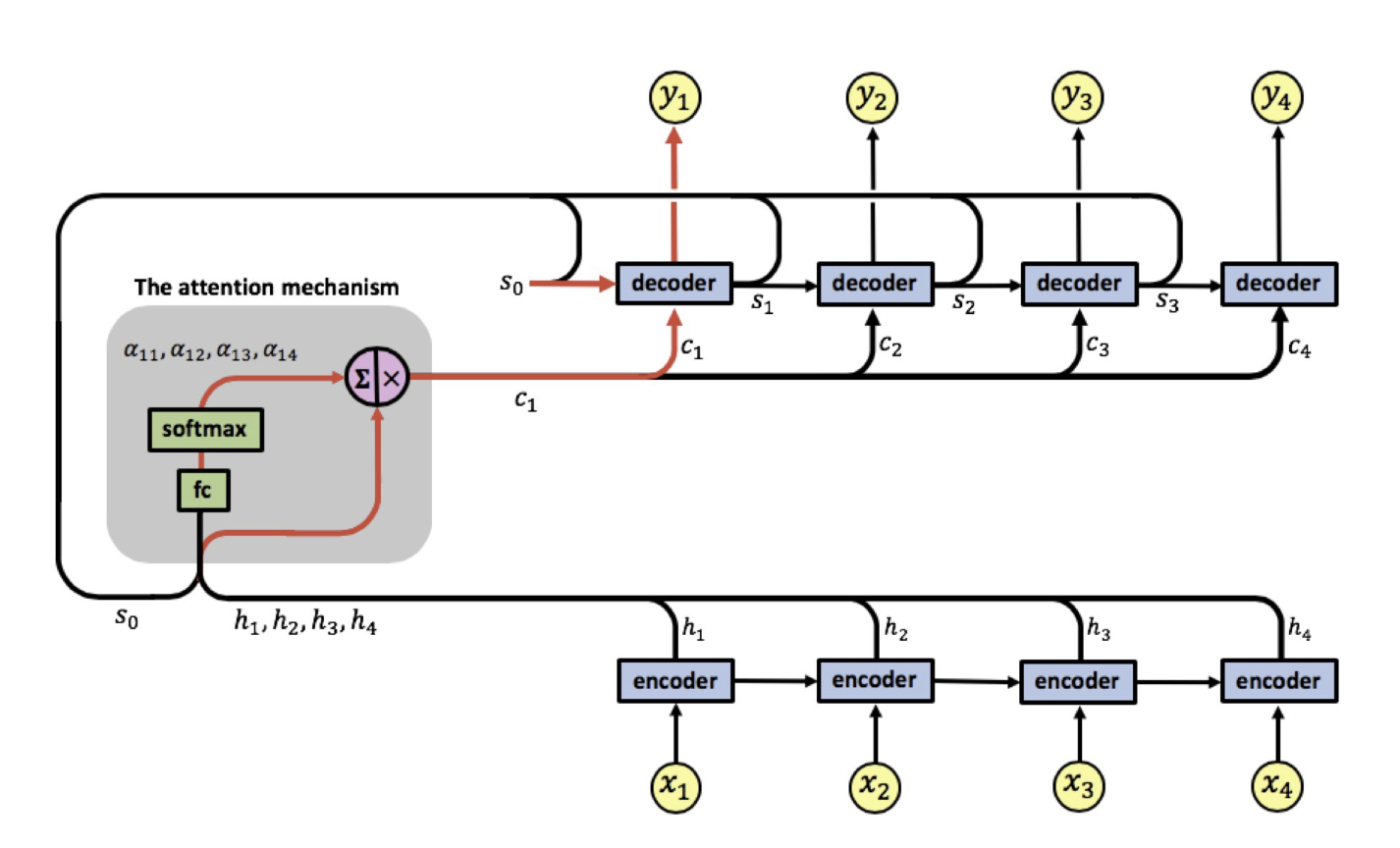
The attention mechanism picks up the inputs and computes the first set of attention weights $\alpha_{11}, \alpha_{12}, \alpha_{13}, \alpha_{14}$ enabling the computation of the first context vector $c_1$. The decoder now uses $[s_0,c_1]$ to generate the first output $y_1$. This process then repeats itself, until we've generated all the outputs.
Data Preparation
This part is pretty much identical to that of the vanilla seq2seq, hence explanation is omitted.
# !python -m spacy download de
# !python -m spacy download en
SEED = 2222
random.seed(SEED)
torch.manual_seed(SEED)
# tokenize sentences into individual tokens
# https://spacy.io/usage/spacy-101#annotations-token
spacy_de = spacy.load('de_core_news_sm')
spacy_en = spacy.load('en_core_web_sm')

def tokenize_de(text):
    return [tok.text for tok in spacy_de.tokenizer(text)][::-1]

def tokenize_en(text):
    return [tok.text for tok in spacy_en.tokenizer(text)]
source = Field(tokenize=tokenize_de, init_token='<sos>', eos_token='<eos>', lower=True)
target = Field(tokenize=tokenize_en, init_token='<sos>', eos_token='<eos>', lower=True)
train_data, valid_data, test_data = Multi30k.splits(exts=('.de', '.en'), fields=(source, target))
print(f"Number of training examples: {len(train_data.examples)}")
print(f"Number of validation examples: {len(valid_data.examples)}")
print(f"Number of testing examples: {len(test_data.examples)}")
train_data.examples[0].src
train_data.examples[0].trg
source.build_vocab(train_data, min_freq=2)
target.build_vocab(train_data, min_freq=2)
print(f"Unique tokens in source (de) vocabulary: {len(source.vocab)}")
print(f"Unique tokens in target (en) vocabulary: {len(target.vocab)}")
device = torch.device('cuda' if torch.cuda.is_available() else 'cpu')
BATCH_SIZE = 128

# create batches out of the dataset and sends them to the appropriate device
train_iterator, valid_iterator, test_iterator = BucketIterator.splits(
    (train_data, valid_data, test_data), batch_size=BATCH_SIZE, device=device)
test_batch = next(iter(test_iterator))
test_batch
Model Implementation
# adjustable parameters
INPUT_DIM = len(source.vocab)
OUTPUT_DIM = len(target.vocab)
ENC_EMB_DIM = 256
DEC_EMB_DIM = 256
ENC_HID_DIM = 512
DEC_HID_DIM = 512
N_LAYERS = 1
ENC_DROPOUT = 0.5
DEC_DROPOUT = 0.5
The following sections are heavily "borrowed" from the wonderful tutorial on this topic listed below.
Some personal preference modifications have been made.
Encoder
Like other seq2seq-like architectures, we first need to specify an encoder. Here we'll be using a bidirectional GRU layer. With a bidirectional layer, we have a forward layer scanning the sentence from left to right (shown below in green), and a backward layer scanning the sentence from right to left (yellow). From the coding perspective, we need to set the bidirectional=True for the GRU layer's argument.

More formally, we now have:
$$ \begin{align} h_t^\rightarrow &= \text{EncoderGRU}^\rightarrow(x_t^\rightarrow,h_{t-1}^\rightarrow)\\ h_t^\leftarrow &= \text{EncoderGRU}^\leftarrow(x_t^\leftarrow,h_{t-1}^\leftarrow) \end{align} $$Where $x_0^\rightarrow = \text{<sos>}, x_1^\rightarrow = \text{guten}$ and $x_0^\leftarrow = \text{<eos>}, x_1^\leftarrow = \text{morgen}$.
As before, we only pass an embedded input to our GRU layer. We'll get two context vectors, one from the forward layer after it has seen the final word in the sentence, $z^\rightarrow=h_T^\rightarrow$, and one from the backward layer after it has seen the first word in the sentence, $z^\leftarrow=h_T^\leftarrow$.
As we'll be using bidirectional layer, the next section is devoted to help us understand how the output looks like before we implement the actual encoder that we'll be using. The shape of the output is explicitly printed out to make it easier to comprehend. Here, we're using GRU layer, which can be replaced with a LSTM layer, which is similar, but return an additional cell state variable that has the same size as the hidden state.
class Encoder(nn.Module):
    def __init__(self, input_dim, emb_dim, hid_dim, n_layers, dropout):
        super().__init__()
        self.emb_dim = emb_dim
        self.hid_dim = hid_dim
        self.input_dim = input_dim
        self.n_layers = n_layers
        self.dropout = dropout

        self.embedding = nn.Embedding(input_dim, emb_dim)
        self.rnn = nn.GRU(emb_dim, hid_dim, n_layers, dropout=dropout,
                          bidirectional=True)

    def forward(self, src_batch):
        # src [sent len, batch size]
        embedded = self.embedding(src_batch) # [sent len, batch size, emb dim]
        outputs, hidden = self.rnn(embedded)  # [sent len, batch size, hidden dim]
        # outputs -> [sent len, batch size, hidden dim * n directions]
        # hidden -> [n layers * n directions, batch size, hidden dim]
        return outputs, hidden
# first experiment with n_layers = 1
n_layers = 1
encoder = Encoder(INPUT_DIM, ENC_EMB_DIM, ENC_HID_DIM, n_layers, ENC_DROPOUT).to(device)
outputs, hidden = encoder(test_batch.src)
outputs.shape, hidden.shape
Notice that output's last dimension is 1024, which is the hidden dimension (512) multiplied by the number of directions (2). Whereas the hidden's first dimension is 2, representing the number of directions (2).
- The returned outputs of bidirectional RNN at timestep $t$ is the output after feeding input to both the reverse and normal RNN unit at timestep $t$, where normal RNN has seen inputs $1...t$ and reverse RNN has seen inputs $t...n$, with $n$ being the length of the sequence).
- The returned hidden state of bidirectional RNN is the hidden state after the whole sequence is consume. For normal RNN it's after timestep $n$; for reverse RNN it's after timestep 1.
The following diagram can also come in handy when visualizing the difference between output and hidden.
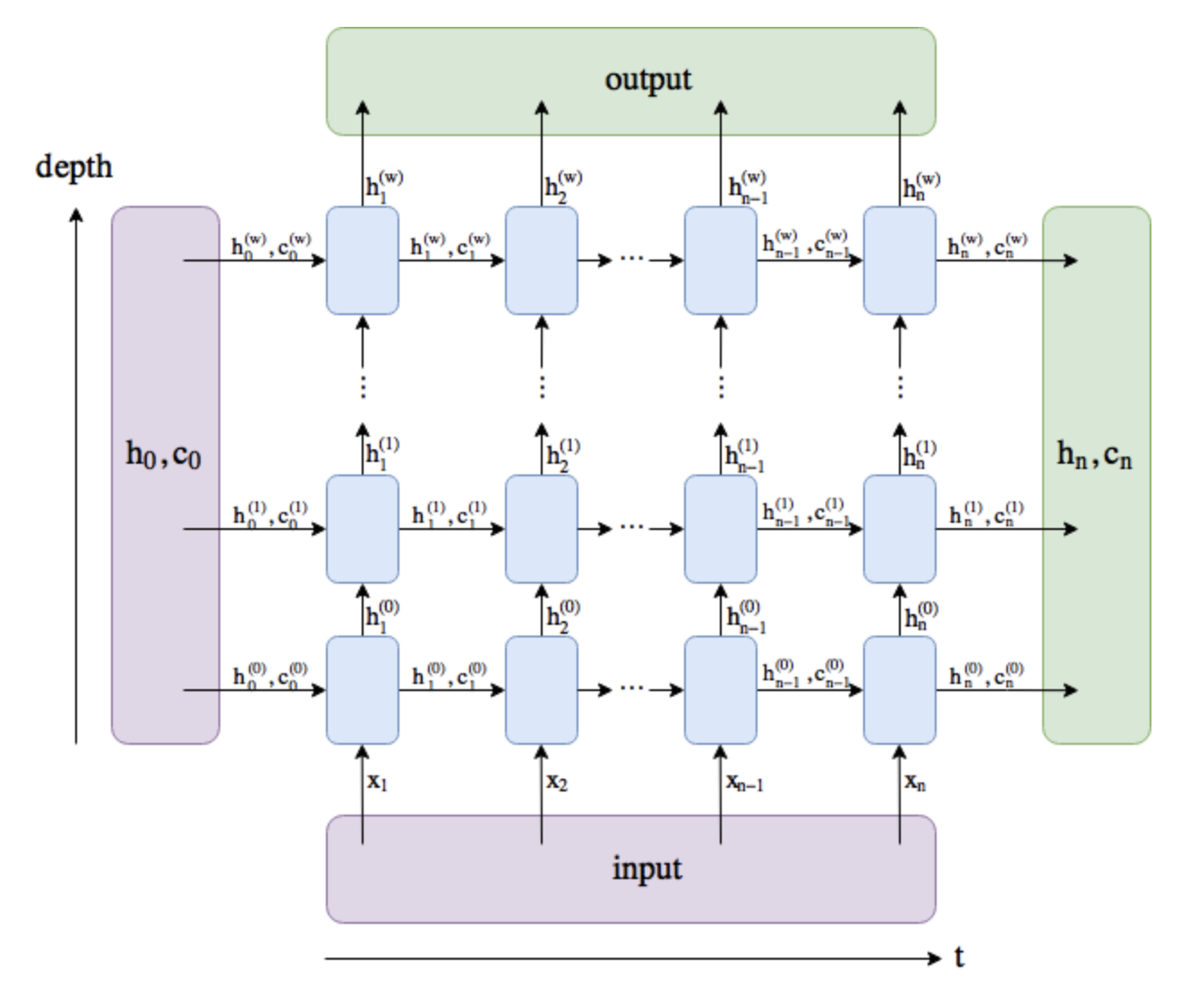
In the diagram $n$ notes each timestep, and $w$ denotes the number of layer.
- output comprises all the hidden states in the last layer ("last" depth-wise, not time-wise).
- ($h_n$, $c_n$) comprise of the hidden states after the last timestep, $t = n$, so we could potentially feed them into another LSTM layer.
# the outputs are concatenated at the last dimension
assert (outputs[-1, :, :ENC_HID_DIM] == hidden[0]).all()
assert (outputs[0, :, ENC_HID_DIM:] == hidden[1]).all()
# experiment with n_layers = 2
n_layers = 2
encoder = Encoder(INPUT_DIM, ENC_EMB_DIM, ENC_HID_DIM, n_layers, ENC_DROPOUT).to(device)
outputs, hidden = encoder(test_batch.src)
outputs.shape, hidden.shape
Notice now the first dimension of the hidden cell becomes 4, which represents the number of layers (2) multiplied by the number of directions (2). The order of the hidden state is stacked by [forward_1, backward_1, forward_2, backward_2, ...]
assert (outputs[-1, :, :ENC_HID_DIM] == hidden[2]).all()
assert (outputs[0, :, ENC_HID_DIM:] == hidden[3]).all()
We'll need some final touches for our actual encoder. As our encoder's hidden state will be used as the decoder's initial hidden state, we need to make sure we make them the same shape. In our example, the decoder is not bidirectional, and only needs a single context vector, $z$, to use as its initial hidden state, $s_0$, and we currently have two, a forward and a backward one ($z^\rightarrow=h_T^\rightarrow$ and $z^\leftarrow=h_T^\leftarrow$, respectively). We solve this by concatenating the two context vectors together, passing them through a linear layer, $g$, and applying the $\tanh$ activation function.
$$ \begin{align} z=\tanh(g(h_T^\rightarrow, h_T^\leftarrow)) = \tanh(g(z^\rightarrow, z^\leftarrow)) = s_0 \end{align} $$class Encoder(nn.Module):
def __init__(self, input_dim, emb_dim, enc_hid_dim, dec_hid_dim, n_layers, dropout):
super().__init__()
self.emb_dim = emb_dim
self.enc_hid_dim = enc_hid_dim
self.dec_hid_dim = dec_hid_dim
self.input_dim = input_dim
self.n_layers = n_layers
self.dropout = dropout
self.embedding = nn.Embedding(input_dim, emb_dim)
self.rnn = nn.GRU(emb_dim, enc_hid_dim, n_layers, dropout=dropout,
bidirectional=True)
self.fc = nn.Linear(enc_hid_dim * 2, dec_hid_dim)
def forward(self, src_batch):
# src [sent len, batch size]
# [sent len, batch size, emb dim]
embedded = self.embedding(src_batch)
outputs, hidden = self.rnn(embedded)
# outputs -> [sent len, batch size, hidden dim * n directions]
# hidden -> [n layers * n directions, batch size, hidden dim]
# initial decoder hidden is final hidden state of the forwards and
# backwards encoder RNNs fed through a linear layer
concated = torch.cat((hidden[-2, :, :], hidden[-1, :, :]), dim=1)
hidden = torch.tanh(self.fc(concated))
return outputs, hidden
encoder = Encoder(INPUT_DIM, ENC_EMB_DIM, ENC_HID_DIM, DEC_HID_DIM, N_LAYERS, ENC_DROPOUT).to(device)
outputs, hidden = encoder(test_batch.src)
outputs.shape, hidden.shape
Attention
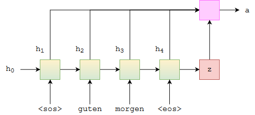
The next part is the hightlight. The attention layer will take in the previous hidden state of the decoder $s_{t-1}$, and all of the stacked forward and backward hidden state from the encoder $H$. The output will be an attention vector $a_t$, that is the length of the source sentece, each element of this vector will be a floating number between 0 and 1, and the entire vector sums up to 1.
Intuitively, this layer takes in what we've decoded so far $s_{t-1}$, and all of what have encoded $H$, to produce a vector $a_t$, that represents which word in the source sentence should we pay the most attention to in order to correctly predict the next thing in the target sequence $y_{t+1}$.
Graphically, this looks something like below. For the very first attention vector, where we use the encoder's hidden state as the initial hidden state from the decoder. The green/yellow blocks represent the hidden states from both the forward and backward RNNs, and the attention computation is all done within the pink block.
class Attention(nn.Module):

    def __init__(self, enc_hid_dim, dec_hid_dim):
        super().__init__()
        self.enc_hid_dim = enc_hid_dim
        self.dec_hid_dim = dec_hid_dim

        # enc_hid_dim multiply by 2 due to bidirectional
        self.fc1 = nn.Linear(enc_hid_dim * 2 + dec_hid_dim, dec_hid_dim)
        self.fc2 = nn.Linear(dec_hid_dim, 1, bias=False)

    def forward(self, encoder_outputs, hidden):
        src_len = encoder_outputs.shape[0]
        batch_size = encoder_outputs.shape[1]

        # repeat encoder hidden state src_len times [batch size, sent len, dec hid dim]
        hidden = hidden.unsqueeze(1).repeat(1, src_len, 1)
        # reshape/permute the encoder output, so that the batch size comes first
        # [batch size, sent len, enc hid dim * 2], times 2 because of bidirectional
        outputs = encoder_outputs.permute(1, 0, 2)

        # the attention mechanism receives a concatenation of the hidden state
        # and the encoder output
        concat = torch.cat((hidden, outputs), dim=2)

        # fully connected layer and softmax layer to compute the attention weight
        # [batch size, sent len, dec hid dim]
        energy = torch.tanh(self.fc1(concat))

        # attention weight should be of [batch size, sent len]
        attention = self.fc2(energy).squeeze(dim=2)
        attention_weight = torch.softmax(attention, dim=1)
        return attention_weight
attention = Attention(ENC_HID_DIM, DEC_HID_DIM).to(device)
attention_weight = attention(outputs, hidden)
attention_weight.shape
Decoder
Now comes the decoder, within the decoder, we first use the attention layer that we've created in the previous section to compute the attention weight, this gives us the weight for each source sentence that the model should pay attention to when generating the current target output in the sequence. Along with the output from the encoder, this gives us the context vector. Finally, the decoder takes the embedded input along with the context to generate the target output in the sequence.
class Decoder(nn.Module):

    def __init__(self, output_dim, emb_dim, enc_hid_dim, dec_hid_dim, n_layers,
                 dropout, attention):
        super().__init__()
        self.emb_dim = emb_dim
        self.enc_hid_dim = enc_hid_dim
        self.dec_hid_dim = dec_hid_dim
        self.output_dim = output_dim
        self.n_layers = n_layers
        self.dropout = dropout
        self.attention = attention

        self.embedding = nn.Embedding(output_dim, emb_dim)
        self.rnn = nn.GRU(enc_hid_dim * 2 + emb_dim, dec_hid_dim, n_layers, dropout=dropout)
        self.linear = nn.Linear(dec_hid_dim, output_dim)

    def forward(self, trg, encoder_outputs, hidden):
        # trg [batch size]
        # outputs [src sen len, batch size, enc hid dim * 2], times 2 due to bidirectional
        # hidden [batch size, dec hid dim]

        # [batch size, 1, sent len]
        attention = self.attention(encoder_outputs, hidden).unsqueeze(1)

        # [batch size, sent len, enc hid dim * 2]
        outputs = encoder_outputs.permute(1, 0, 2)

        # [1, batch size, enc hid dim * 2]
        context = torch.bmm(attention, outputs).permute(1, 0, 2)

        # input sentence -> embedding
        # [1, batch size, emb dim]
        embedded = self.embedding(trg.unsqueeze(0))
        rnn_input = torch.cat((embedded, context), dim=2)

        outputs, hidden = self.rnn(rnn_input, hidden.unsqueeze(0))
        prediction = self.linear(outputs.squeeze(0))
        return prediction, hidden.squeeze(0)
decoder = Decoder(OUTPUT_DIM, DEC_EMB_DIM, ENC_HID_DIM, DEC_HID_DIM, N_LAYERS, DEC_DROPOUT, attention).to(device)
prediction, decoder_hidden = decoder(test_batch.trg[0], outputs, hidden)

# notice the decoder_hidden's shape should match the shape that's generated by
# the encoder
prediction.shape, decoder_hidden.shape
Seq2Seq
This part is about putting the encoder and decoder together and is very much identical to the vanilla seq2seq framework, hence the explanation is omitted.
class Seq2Seq(nn.Module):
    def __init__(self, encoder, decoder, device):
        super().__init__()
        self.encoder = encoder
        self.decoder = decoder
        self.device = device

    def forward(self, src_batch, trg_batch, teacher_forcing_ratio=0.5):
        max_len, batch_size = trg_batch.shape
        trg_vocab_size = self.decoder.output_dim

        # tensor to store decoder's output
        outputs = torch.zeros(max_len, batch_size, trg_vocab_size).to(self.device)

        # encoder_outputs : all hidden states of the input sequence (forward and backward)
        # hidden : final forward and backward hidden states, passed through a linear layer
        encoder_outputs, hidden = self.encoder(src_batch)

        trg = trg_batch[0]
        for i in range(1, max_len):
            prediction, hidden = self.decoder(trg, encoder_outputs, hidden)
            outputs[i] = prediction

            if random.random() < teacher_forcing_ratio:
                trg = trg_batch[i]
            else:
                trg = prediction.argmax(1)

        return outputs
attention = Attention(ENC_HID_DIM, DEC_HID_DIM)
encoder = Encoder(INPUT_DIM, ENC_EMB_DIM, ENC_HID_DIM, DEC_HID_DIM, N_LAYERS, ENC_DROPOUT)
decoder = Decoder(OUTPUT_DIM, DEC_EMB_DIM, ENC_HID_DIM, DEC_HID_DIM, N_LAYERS, DEC_DROPOUT, attention)
seq2seq = Seq2Seq(encoder, decoder, device).to(device)
seq2seq
outputs = seq2seq(test_batch.src, test_batch.trg)
outputs.shape
def count_parameters(model):
    return sum(p.numel() for p in model.parameters() if p.requires_grad)

print(f'The model has {count_parameters(seq2seq):,} trainable parameters')
Training Seq2Seq
We've done the hard work of defining our seq2seq module. The final touch is to specify the training/evaluation loop.
optimizer = optim.Adam(seq2seq.parameters())

# ignore the padding index when calculating the loss
PAD_IDX = target.vocab.stoi['<pad>']
criterion = nn.CrossEntropyLoss(ignore_index=PAD_IDX)
def train(seq2seq, iterator, optimizer, criterion):
    seq2seq.train()

    epoch_loss = 0
    for batch in iterator:
        optimizer.zero_grad()
        outputs = seq2seq(batch.src, batch.trg)

        # the loss function only works on 2d inputs
        # and 1d targets we need to flatten each of them
        outputs_flatten = outputs[1:].view(-1, outputs.shape[-1])
        trg_flatten = batch.trg[1:].view(-1)
        loss = criterion(outputs_flatten, trg_flatten)

        loss.backward()
        optimizer.step()

        epoch_loss += loss.item()

    return epoch_loss / len(iterator)
def evaluate(seq2seq, iterator, criterion):
    seq2seq.eval()

    epoch_loss = 0
    with torch.no_grad():
        for batch in iterator:
            # turn off teacher forcing
            outputs = seq2seq(batch.src, batch.trg, teacher_forcing_ratio=0)

            # trg = [trg sent len, batch size]
            # output = [trg sent len, batch size, output dim]
            outputs_flatten = outputs[1:].view(-1, outputs.shape[-1])
            trg_flatten = batch.trg[1:].view(-1)
            loss = criterion(outputs_flatten, trg_flatten)
            epoch_loss += loss.item()

    return epoch_loss / len(iterator)
def epoch_time(start_time, end_time):
    elapsed_time = end_time - start_time
    elapsed_mins = int(elapsed_time / 60)
    elapsed_secs = int(elapsed_time - (elapsed_mins * 60))
    return elapsed_mins, elapsed_secs
N_EPOCHS = 10
best_valid_loss = float('inf')

for epoch in range(N_EPOCHS):
    start_time = time.time()
    train_loss = train(seq2seq, train_iterator, optimizer, criterion)
    valid_loss = evaluate(seq2seq, valid_iterator, criterion)
    end_time = time.time()

    epoch_mins, epoch_secs = epoch_time(start_time, end_time)

    if valid_loss < best_valid_loss:
        best_valid_loss = valid_loss
        torch.save(seq2seq.state_dict(), 'tut2-model.pt')

    print(f'Epoch: {epoch+1:02} | Time: {epoch_mins}m {epoch_secs}s')
    print(f'\tTrain Loss: {train_loss:.3f} | Train PPL: {math.exp(train_loss):7.3f}')
    print(f'\t Val. Loss: {valid_loss:.3f} |  Val. PPL: {math.exp(valid_loss):7.3f}')
Evaluating Seq2Seq
seq2seq.load_state_dict(torch.load('tut2-model.pt'))

test_loss = evaluate(seq2seq, test_iterator, criterion)
print(f'| Test Loss: {test_loss:.3f} | Test PPL: {math.exp(test_loss):7.3f} |')
Here, we pick a random example in our dataset, print out the original source and target sentence. Then takes a look at whether the "predicted" target sentence generated by the model.
example_idx = 0
example = train_data.examples[example_idx]
print('source sentence: ', ' '.join(example.src))
print('target sentence: ', ' '.join(example.trg))
src_tensor = source.process([example.src]).to(device)
trg_tensor = target.process([example.trg]).to(device)
print(trg_tensor.shape)

seq2seq.eval()
with torch.no_grad():
    outputs = seq2seq(src_tensor, trg_tensor, teacher_forcing_ratio=0)

outputs.shape
output_idx = outputs[1:].squeeze(1).argmax(1)
' '.join([target.vocab.itos[idx] for idx in output_idx])
Summary
- Upon implementing the attention mechanism, we were able to achieve a better evaluation score on the test set, while even using less parameters. As mentioned in the original paper:
We extended the basic encoder–decoder by letting a model (soft)search for a set of input words. This frees the model from having to encode the whole source sentence into a fixed-length vector, and also lets the model focus only on information relevant to the generation of the next target word. This has a major positive impact on the ability of the neural machine translation system to yield good results on longer sentences.
- Note that another interesting thing that we're capable of doing but wasn't done here is to visualize the attention weight to see for a given translation, where the model is focusing on.
Reference
- Blog: Attention in RNNs
- Stackoverflow: What's the difference between “hidden” and “output” in PyTorch LSTM?
- Jupyter Notebook: Neural Machine Translation by Jointly Learning to Align and Translate
- Paper: D. Bahdanau, K. Cho, Y. Bengio (2014) - Neural Machine Translation by Jointly Learning to Align and Translate