Table of Contents
# code for loading the format for the notebook
import os

# path : store the current path to convert back to it later
path = os.getcwd()
os.chdir(os.path.join('..', '..', 'notebook_format'))

from formats import load_style
load_style(css_style='custom2.css', plot_style=False)
os.chdir(path)

# 1. magic for inline plot
# 2. magic to print version
# 3. magic so that the notebook will reload external python modules
# 4. magic to enable retina (high resolution) plots
# https://gist.github.com/minrk/3301035
%matplotlib inline
%load_ext watermark
%load_ext autoreload
%autoreload 2
%config InlineBackend.figure_format='retina'

import os
import math
import time
import spacy
import torch
import random
import numpy as np
import torch.nn as nn
import torch.optim as optim
from typing import List
from torchtext.datasets import Multi30k
from torchtext.data import Field, BucketIterator

%watermark -a 'Ethen' -d -t -v -p numpy,torch,torchtext,spacy
Seq2Seq
Seq2Seq (Sequence to Sequence) is a many to many network where two neural networks, one encoder and one decoder work together to transform one sequence to another. The core highlight of this method is having no restrictions on the length of the source and target sequence. At a high-level, the way it works is:
- The encoder network condenses an input sequence into a vector, this vector is a smaller dimensional representation and is often referred to as the context/thought vector. This thought vector is served as an abstract representation for the entire input sequence.
- The decoder network takes in that thought vector and unfolds that vector into the output sequence.
The main use case includes:
- chatbots
- text summarization
- speech recognition
- image captioning
- machine translation
In this notebook, we'll be implementing the seq2seq model ourselves using Pytorch and use it in the context of German to English translations.
Seq2Seq Introduction
The following sections are heavily "borrowed" from the wonderful tutorial on this topic listed below.
Some personal preference modifications have been made.
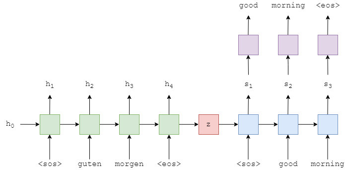
The above image shows an example translation. The input/source sentence, "guten morgen", is input into the encoder (green) one word at a time. We also append a start of sequence (<sos>) and end of sequence (<eos>) token to the start and end of sentence, respectively. At each time-step, the input to the encoder is both the current word, $x_t$, as well as the hidden state from the previous time-step, $h_{t-1}$, and the encoder outputs a new hidden state $h_t$. We can think of the hidden state as a vector representation of the sentence so far. The can be represented as a function of both of $x_t$ and $h_{t-1}$:
We're using the term encoder loosely here, in practice, it can be any type of architecture, the most common ones being RNN-type network such as LSTM (Long Short-Term Memory) or a GRU (Gated Recurrent Unit).
Here, we have $X = \{x_1, x_2, ..., x_T\}$, where $x_1 = \text{<sos>}, x_2 = \text{guten}$, etc. The initial hidden state, $h_0$, is usually either initialized to zeros or a learned parameter.
Once the final word, $x_T$, has been passed into the encoder, we use the final hidden state, $h_T$, as the context vector, i.e. $h_T = z$. This is a vector representation of the entire source sentence.
Now we have our context vector, $z$, we can start decoding it to get the target sentence, "good morning". Again, we append the start and end of sequence tokens to the target sentence. At each time-step, the input to the decoder (blue) is the current word, $y_t$, as well as the hidden state from the previous time-step, $s_{t-1}$, where the initial decoder hidden state, $s_0$, is the context vector, $s_0 = z = h_T$, i.e. the initial decoder hidden state is the final encoder hidden state. Thus, similar to the encoder, we can represent the decoder as:
$$s_t = \text{Decoder}(y_t, s_{t-1})$$In the decoder, we need to go from the hidden state to an actual word, therefore at each time-step we use $s_t$ to predict (by passing it through a Linear layer, shown in purple) what we think is the next word in the sequence, $\hat{y}_t$.
The words in the decoder are always generated one after another, with one per time-step. We always use <sos> for the first input to the decoder, $y_1$, but for subsequent inputs, $y_{t>1}$, we will sometimes use the actual, ground truth next word in the sequence, $y_t$ and sometimes use the word predicted by our decoder, $\hat{y}_{t-1}$. This is called teacher forcing, which we'll later see in action.
When training/testing our model, we always know how many words are in our target sentence, so we stop generating words once we hit that many. During inference (i.e. real world usage) it is common to keep generating words until the model outputs an <eos> token or after a certain amount of words have been generated.
Once we have our predicted target sentence, $\hat{Y} = \{ \hat{y}_1, \hat{y}_2, ..., \hat{y}_T \}$, we compare it against our actual target sentence, $Y = \{ y_1, y_2, ..., y_T \}$, to calculate our loss. We then use this loss to update all of the parameters in our model.
Data Preparation
We'll be coding up the models in PyTorch and using TorchText to help us do all of the pre-processing required. We'll also be using spaCy to assist in the tokenization of the data. We will introduce the functionalities some these libraries along the way as well.
SEED = 2222
random.seed(SEED)
torch.manual_seed(SEED)
The next two code chunks:
- Downloads the spacy model for the German and English language.
- Create the tokenizer functions, which will take in the sentence as the input and return the sentence as a list of tokens. These functions can then be passed to torchtext.
# !python -m spacy download de
# !python -m spacy download en
# the link below contains explanation of how spacy's tokenization works
# https://spacy.io/usage/spacy-101#annotations-token
spacy_de = spacy.load('de_core_news_sm')
spacy_en = spacy.load('en_core_web_sm')


def tokenize_de(text: str) -> List[str]:
    return [tok.text for tok in spacy_de.tokenizer(text)][::-1]

def tokenize_en(text: str) -> List[str]:
    return [tok.text for tok in spacy_en.tokenizer(text)]
text = "I don't like apple."
tokenize_en(text)
The tokenizer is language specific, e.g. it knows that in the English language don't should be tokenized into do not (n't).
Another thing to note is that the order of the source sentence is reversed during the tokenization process. The rationale behind things comes from the original seq2seq paper where they identified that this trick improved the result of their model.
Normally, when we concatenate a source sentence with a target sentence, each word in the source sentence is far from its corresponding word in the target sentence. By reversing the source sentence, the first few words in the source sentence now becomes very close to the first few words in the target sentence, thus the model would have lesser issue establishing communication between the source and target sentence. Although, the average distance between words in the source and target language remains the same during this process, however, it was shown that the model learned much better even on later parts of the sentence.
Declaring Fields
Moving on, we will begin leveraging torchtext's functionality. The first once is Field, which is where we specify how we wish to preprocess our text data for a certain field.
Here, we set the tokenize argument to the correct tokenization function for the source and target field, with German being the source field and English being the target field. The field also appends the "start of sequence" and "end of sequence" tokens via the init_token and eos_token arguments, and converts all words to lowercase. The docstring of the Field object is pretty well-written, please refer to it to see other arguments that it takes in.
source = Field(tokenize=tokenize_de, init_token='<sos>', eos_token='<eos>', lower=True)
target = Field(tokenize=tokenize_en, init_token='<sos>', eos_token='<eos>', lower=True)
Constructing Dataset
We've defined the logic of processing our raw text data, now we need to tell the fields what data it should work on. This is where Dataset comes in. The dataset we'll be using is the Multi30k dataset. This is a dataset with ~30,000 parallel English, German and French sentences, each with ~12 words per sentence. Torchtext comes with a capability for us to download and load the training, validation and test data.
exts specifies which languages to use as the source and target (source goes first) and fields specifies which field to use for the source and target.
train_data, valid_data, test_data = Multi30k.splits(exts=('.de', '.en'), fields=(source, target))
print(f"Number of training examples: {len(train_data.examples)}")
print(f"Number of validation examples: {len(valid_data.examples)}")
print(f"Number of testing examples: {len(test_data.examples)}")
Upon loading the dataset, we can indexed and iterate over the Dataset like a normal list. Each element in the dataset bundles the attributes of a single record for us. We can index our dataset like a list and then access the .src and .trg attribute to take a look at the tokenized source and target sentence.
# equivalent, albeit more verbiage train_data.examples[0].src
train_data[0].src
train_data[0].trg
The next missing piece is to build the vocabulary for the source and target languages. That way we can convert our tokenized tokens into integers so that they can be fed into downstream models. Constructing the vocabulary and word to integer mapping is done by calling the build_vocab method of a Field on a dataset. This adds the vocab attribute to the field.
The vocabularies of the source and target languages are distinct. Using the min_freq argument, we only allow tokens that appear at least 2 times to appear in our vocabulary. Tokens that appear only once are converted into an <unk> (unknown) token (we can customize this in the Field earlier if we like).
It is important to note that our vocabulary should only be built from the training set and not the validation/test set. This prevents "information leakage" into our model, giving us artificially inflated validation/test scores.
source.build_vocab(train_data, min_freq=2)
target.build_vocab(train_data, min_freq=2)
print(f"Unique tokens in source (de) vocabulary: {len(source.vocab)}")
print(f"Unique tokens in target (en) vocabulary: {len(target.vocab)}")
Constructing Iterator
The final step of preparing the data is to create the iterators. Very similar to DataLoader in the standard pytorch package, Iterator in torchtext converts our data into batches, so that they can be fed into the model. These can be iterated on to return a batch of data which will have a src and trg attribute (PyTorch tensors containing a batch of numericalized source and target sentences). Numericalized is just a fancy way of saying they have been converted from a sequence of tokens to a sequence of corresponding indices, where the mapping between the tokens and indices comes from the learned vocabulary.
When we get a batch of examples using an iterator we need to make sure that all of the source sentences are padded to the same length, the same with the target sentences. Luckily, torchtext iterators handle this for us! BucketIterator is a extremely useful torchtext feature. It automatically shuffles and buckets the input sequences into sequences of similar length, this minimizes the amount of padding that we need to perform.
BATCH_SIZE = 128

# pytorch boilerplate that determines whether a GPU is present or not,
# this determines whether our dataset or model can to moved to a GPU
device = torch.device('cuda' if torch.cuda.is_available() else 'cpu')

# create batches out of the dataset and sends them to the appropriate device
train_iterator, valid_iterator, test_iterator = BucketIterator.splits(
    (train_data, valid_data, test_data), batch_size=BATCH_SIZE, device=device)
# pretend that we're iterating over the iterator and print out the print element
test_batch = next(iter(test_iterator))
test_batch
test_batch.src
We can list out the first batch, we see each element of the iterator is a Batch object, similar to element of a Dataset, we can access the fields via its attributes. The next important thing to note that it is of size [sentence length, batch size], and the longest sentence in the first batch of the source language has a length of 10.
Seq2Seq Implementation
# adjustable parameters
INPUT_DIM = len(source.vocab)
OUTPUT_DIM = len(target.vocab)
ENC_EMB_DIM = 256
DEC_EMB_DIM = 256
HID_DIM = 512
N_LAYERS = 2
ENC_DROPOUT = 0.5
DEC_DROPOUT = 0.5
To define our seq2seq model, we first specify the encoder and decoder separately.
Encoder Module
class Encoder(nn.Module):
    """
    Input :
        - source batch
    Layer :
        source batch -> Embedding -> LSTM
    Output :
        - LSTM hidden state
        - LSTM cell state

    Parmeters
    ---------
    input_dim : int
        Input dimension, should equal to the source vocab size.

    emb_dim : int
        Embedding layer's dimension.

    hid_dim : int
        LSTM Hidden/Cell state's dimension.

    n_layers : int
        Number of LSTM layers.

    dropout : float
        Dropout for the LSTM layer.
    """

    def __init__(self, input_dim: int, emb_dim: int, hid_dim: int, n_layers: int, dropout: float):
        super().__init__()
        self.emb_dim = emb_dim
        self.hid_dim = hid_dim
        self.input_dim = input_dim
        self.n_layers = n_layers
        self.dropout = dropout

        self.embedding = nn.Embedding(input_dim, emb_dim)
        self.rnn = nn.LSTM(emb_dim, hid_dim, n_layers, dropout=dropout)

    def forward(self, src_batch: torch.LongTensor):
        """

        Parameters
        ----------
        src_batch : 2d torch.LongTensor
            Batched tokenized source sentence of shape [sent len, batch size].

        Returns
        -------
        hidden, cell : 3d torch.LongTensor
            Hidden and cell state of the LSTM layer. Each state's shape
            [n layers * n directions, batch size, hidden dim]
        """
        embedded = self.embedding(src_batch) # [sent len, batch size, emb dim]
        outputs, (hidden, cell) = self.rnn(embedded)
        # outputs -> [sent len, batch size, hidden dim * n directions]
        return hidden, cell
encoder = Encoder(INPUT_DIM, ENC_EMB_DIM, HID_DIM, N_LAYERS, ENC_DROPOUT).to(device)
hidden, cell = encoder(test_batch.src)
hidden.shape, cell.shape
Decoder Module
The decoder accept a batch of input tokens, previous hidden states and previous cell states. Note that in the decoder module, we are only decoding one token at a time, the input tokens will always have a sequence length of 1. This is different from the encoder module where we encode the entire source sentence all at once.
class Decoder(nn.Module):
    """
    Input :
        - first token in the target batch
        - LSTM hidden state from the encoder
        - LSTM cell state from the encoder
    Layer :
        target batch -> Embedding --
                                   |
        encoder hidden state ------|--> LSTM -> Linear
                                   |
        encoder cell state   -------

    Output :
        - prediction
        - LSTM hidden state
        - LSTM cell state

    Parmeters
    ---------
    output : int
        Output dimension, should equal to the target vocab size.

    emb_dim : int
        Embedding layer's dimension.

    hid_dim : int
        LSTM Hidden/Cell state's dimension.

    n_layers : int
        Number of LSTM layers.

    dropout : float
        Dropout for the LSTM layer.
    """

    def __init__(self, output_dim: int, emb_dim: int, hid_dim: int, n_layers: int, dropout: float):
        super().__init__()
        self.emb_dim = emb_dim
        self.hid_dim = hid_dim
        self.output_dim = output_dim
        self.n_layers = n_layers
        self.dropout = dropout

        self.embedding = nn.Embedding(output_dim, emb_dim)
        self.rnn = nn.LSTM(emb_dim, hid_dim, n_layers, dropout=dropout)
        self.out = nn.Linear(hid_dim, output_dim)

    def forward(self, trg: torch.LongTensor, hidden: torch.FloatTensor, cell: torch.FloatTensor):
        """

        Parameters
        ----------
        trg : 1d torch.LongTensor
            Batched tokenized source sentence of shape [batch size].

        hidden, cell : 3d torch.FloatTensor
            Hidden and cell state of the LSTM layer. Each state's shape
            [n layers * n directions, batch size, hidden dim]

        Returns
        -------
        prediction : 2d torch.LongTensor
            For each token in the batch, the predicted target vobulary.
            Shape [batch size, output dim]

        hidden, cell : 3d torch.FloatTensor
            Hidden and cell state of the LSTM layer. Each state's shape
            [n layers * n directions, batch size, hidden dim]
        """
        # [1, batch size, emb dim], the 1 serves as sent len
        embedded = self.embedding(trg.unsqueeze(0))
        outputs, (hidden, cell) = self.rnn(embedded, (hidden, cell))
        prediction = self.out(outputs.squeeze(0))
        return prediction, hidden, cell
decoder = Decoder(OUTPUT_DIM, DEC_EMB_DIM, HID_DIM, N_LAYERS, DEC_DROPOUT).to(device)

# notice that we are not passing the entire the .trg
prediction, hidden, cell = decoder(test_batch.trg[0], hidden, cell)
prediction.shape, hidden.shape, cell.shape
Seq2Seq Module
For the final part of the implementation, we'll implement the seq2seq model. This will handle:
- receiving the input/source sentence
- using the encoder to produce the context vectors
- using the decoder to produce the predicted output/target sentence
The Seq2Seq model takes in an Encoder, Decoder, and a device (used to place tensors on the GPU, if it exists).
For this implementation, we have to ensure that the number of layers and the hidden (and cell) dimensions are equal in the Encoder and Decoder. This is not always the case, as we do not necessarily need the same number of layers or the same hidden dimension sizes in a sequence-to-sequence model. However, if we do have a different number of layers we will need to make decisions about how this is handled. For example, if our encoder has 2 layers and our decoder only has 1, how is this handled? Do we average the two context vectors output by the decoder? Do we pass both through a linear layer? Do we only use the context vector from the highest layer? etc.
Our forward method takes the source sentence, target sentence and a teacher-forcing ratio. The teacher forcing ratio is used when training our model. When decoding, at each time-step we will predict what the next token in the target sequence will be from the previous tokens decoded. With probability equal to the teaching forcing ratio (teacher_forcing_ratio) we will use the actual ground-truth next token in the sequence as the input to the decoder during the next time-step. However, with probability 1 - teacher_forcing_ratio, we will use the token that the model predicted as the next input to the model, even if it doesn't match the actual next token in the sequence. Note that the teacher forcing ratio is only done during training and should be shut off during evaluation.
The first thing we do in the forward method is to create an outputs tensor that will store all of our predictions, $\hat{Y}$.
We then feed the input/source sentence, $X$/src, into the encoder and receive our final hidden and cell states.
The first input to the decoder is the start of sequence (<sos>) token. As our trg tensor already has the <sos> token appended (all the way back when we defined the init_token in our target field) we get our $y_1$ by slicing into it. We know how long our target sentences should be (max_len), so we loop that many times. During each iteration of the loop, we:
- pass the input, previous hidden and previous cell states ($y_t, s_{t-1}, c_{t-1}$) into the decoder
- receive a prediction, next hidden state and next cell state ($\hat{y}_{t+1}, s_{t}, c_{t}$) from the decoder
- place our prediction, $\hat{y}_{t+1}$/
outputin our tensor of predictions, $\hat{Y}$/outputs - decide if we are going to "teacher force" or not
- if we do, the next
inputis the ground-truth next token in the sequence, $y_{t+1}$/trg[t] - if we don't, the next
inputis the predicted next token in the sequence, $\hat{y}_{t+1}$/top1, which we get by doing anargmaxover the output tensor
- if we do, the next
Once we've made all of our predictions, we return our tensor full of predictions, $\hat{Y}$/outputs.
Note: our decoder loop starts at 1, not 0. This means the 0th element of our outputs tensor remains all zeros. So our trg and outputs look something like:
Later on when we calculate the loss, we cut off the first element of each tensor to get:
$$\begin{align*} \text{trg} = [&y_1, y_2, y_3, <eos>]\\ \text{outputs} = [&\hat{y}_1, \hat{y}_2, \hat{y}_3, <eos>] \end{align*}$$All of this should make more sense after we look at the code in the next few section. Feel free to check out the discussion in these two github issues for some more context with this topic. issue-45 and issue-46
class Seq2Seq(nn.Module):
    def __init__(self, encoder: Encoder, decoder: Decoder, device: torch.device):
        super().__init__()
        self.encoder = encoder
        self.decoder = decoder
        self.device = device

        assert encoder.hid_dim == decoder.hid_dim, \
            'Hidden dimensions of encoder and decoder must be equal!'
        assert encoder.n_layers == decoder.n_layers, \
            'Encoder and decoder must have equal number of layers!'

    def forward(self, src_batch: torch.LongTensor, trg_batch: torch.LongTensor,
                teacher_forcing_ratio: float=0.5):

        max_len, batch_size = trg_batch.shape
        trg_vocab_size = self.decoder.output_dim

        # tensor to store decoder's output
        outputs = torch.zeros(max_len, batch_size, trg_vocab_size).to(self.device)

        # last hidden & cell state of the encoder is used as the decoder's initial hidden state
        hidden, cell = self.encoder(src_batch)

        trg = trg_batch[0]
        for i in range(1, max_len):
            prediction, hidden, cell = self.decoder(trg, hidden, cell)
            outputs[i] = prediction

            if random.random() < teacher_forcing_ratio:
                trg = trg_batch[i]
            else:
                trg = prediction.argmax(1)

        return outputs
# note that this implementation assumes that the size of the hidden layer,
# and the number of layer are the same between the encoder and decoder
encoder = Encoder(INPUT_DIM, ENC_EMB_DIM, HID_DIM, N_LAYERS, ENC_DROPOUT)
decoder = Decoder(OUTPUT_DIM, DEC_EMB_DIM, HID_DIM, N_LAYERS, DEC_DROPOUT)
seq2seq = Seq2Seq(encoder, decoder, device).to(device)
seq2seq
outputs = seq2seq(test_batch.src, test_batch.trg)
outputs.shape
def count_parameters(model):
    return sum(p.numel() for p in model.parameters() if p.requires_grad)

print(f'The model has {count_parameters(seq2seq):,} trainable parameters')
Training Seq2Seq
We've done the hard work of defining our seq2seq module. The final touch is to specify the training/evaluation loop.
optimizer = optim.Adam(seq2seq.parameters())

# ignore the padding index when calculating the loss
PAD_IDX = target.vocab.stoi['<pad>']
criterion = nn.CrossEntropyLoss(ignore_index=PAD_IDX)
def train(seq2seq, iterator, optimizer, criterion):
    seq2seq.train()

    epoch_loss = 0
    for batch in iterator:
        optimizer.zero_grad()
        outputs = seq2seq(batch.src, batch.trg)

        # 1. as mentioned in the seq2seq section, we will
        # cut off the first element when performing the evaluation
        # 2. the loss function only works on 2d inputs
        # with 1d targets we need to flatten each of them
        outputs_flatten = outputs[1:].view(-1, outputs.shape[-1])
        trg_flatten = batch.trg[1:].view(-1)
        loss = criterion(outputs_flatten, trg_flatten)

        loss.backward()
        optimizer.step()

        epoch_loss += loss.item()

    return epoch_loss / len(iterator)
def evaluate(seq2seq, iterator, criterion):
    seq2seq.eval()

    epoch_loss = 0
    with torch.no_grad():
        for batch in iterator:
            # turn off teacher forcing
            outputs = seq2seq(batch.src, batch.trg, teacher_forcing_ratio=0)

            # trg = [trg sent len, batch size]
            # output = [trg sent len, batch size, output dim]
            outputs_flatten = outputs[1:].view(-1, outputs.shape[-1])
            trg_flatten = batch.trg[1:].view(-1)
            loss = criterion(outputs_flatten, trg_flatten)
            epoch_loss += loss.item()

    return epoch_loss / len(iterator)
def epoch_time(start_time, end_time):
    elapsed_time = end_time - start_time
    elapsed_mins = int(elapsed_time / 60)
    elapsed_secs = int(elapsed_time - (elapsed_mins * 60))
    return elapsed_mins, elapsed_secs
N_EPOCHS = 20
best_valid_loss = float('inf')

for epoch in range(N_EPOCHS):
    start_time = time.time()
    train_loss = train(seq2seq, train_iterator, optimizer, criterion)
    valid_loss = evaluate(seq2seq, valid_iterator, criterion)
    end_time = time.time()

    epoch_mins, epoch_secs = epoch_time(start_time, end_time)

    if valid_loss < best_valid_loss:
        best_valid_loss = valid_loss
        torch.save(seq2seq.state_dict(), 'tut1-model.pt')

    # it's easier to see a change in perplexity between epoch as it's an exponential
    # of the loss, hence the scale of the measure is much bigger
    print(f'Epoch: {epoch+1:02} | Time: {epoch_mins}m {epoch_secs}s')
    print(f'\tTrain Loss: {train_loss:.3f} | Train PPL: {math.exp(train_loss):7.3f}')
    print(f'\t Val. Loss: {valid_loss:.3f} |  Val. PPL: {math.exp(valid_loss):7.3f}')
Evaluating Seq2Seq
seq2seq.load_state_dict(torch.load('tut1-model.pt'))

test_loss = evaluate(seq2seq, test_iterator, criterion)
print(f'| Test Loss: {test_loss:.3f} | Test PPL: {math.exp(test_loss):7.3f} |')
Here, we pick a random example in our dataset, print out the original source and target sentence. Then takes a look at whether the "predicted" target sentence generated by the model.
example_idx = 0
example = train_data.examples[example_idx]
print('source sentence: ', ' '.join(example.src))
print('target sentence: ', ' '.join(example.trg))
src_tensor = source.process([example.src]).to(device)
trg_tensor = target.process([example.trg]).to(device)
print(trg_tensor.shape)

seq2seq.eval()
with torch.no_grad():
    outputs = seq2seq(src_tensor, trg_tensor, teacher_forcing_ratio=0)

outputs.shape
output_idx = outputs[1:].squeeze(1).argmax(1)
' '.join([target.vocab.itos[idx] for idx in output_idx])
Summary
In this document:
- We took a stab at implementing a vanilla version of the seq2seq model, and train it on a German to English translation.
- Implemented the trick introduced by the original seq2seq paper where they reverse the order of the tokens in the source sentence.
There are a lot of other tricks/ideas that are mentioned in the original paper and worth exploring. e.g.
- A LSTM with 4 layers was chosen.
- Beam Search was also used to decode the sentence.
- Instead of only relying on log-loss or perplexity, another evaluation metric that they used to evaluate the quality of their translation.
Reference
- Blog: A Comprehensive Introduction to Torchtext (Practical Torchtext part 1)
- Jupyter Notebook: Using TorchText with Your Own Datasets
- Jupyter Notebook: Sequence to Sequence Learning with Neural Networks
- Paper: Sutskever, I., Vinyals, O., and Le, Q. (2014). Sequence to sequence learning with neural networks.