# code for loading the format for the notebook
import os

# path : store the current path to convert back to it later
path = os.getcwd()
os.chdir(os.path.join('..', '..', 'notebook_format'))
from formats import load_style
load_style(css_style = 'custom2.css', plot_style = False)
os.chdir(path)

import os
import warnings
import numpy as np
import tensorflow as tf
from time import time
from keras.datasets import mnist

# 1. magic so that the notebook will reload external python modules
# 2. magic to print version
%load_ext autoreload
%autoreload 2
%load_ext watermark
%watermark -a 'Ethen' -d -t -v -p keras,numpy,tensorflow
LSTM (Long Short Term Memory)
Now that we've understand the motivation behind Recurrent Neural Network (RNN) and seen its implementation. Let's turn our head towards its more powerful variants.
Recall that RNNs are networks with loops in them, allowing them to store information about the previous state and potentially leverage it to better reason about the current state. One popular diagram that we might come across for RNNs is the following:
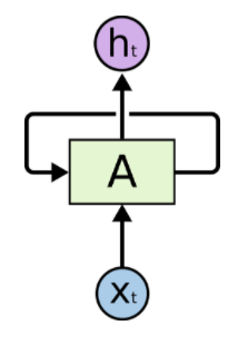
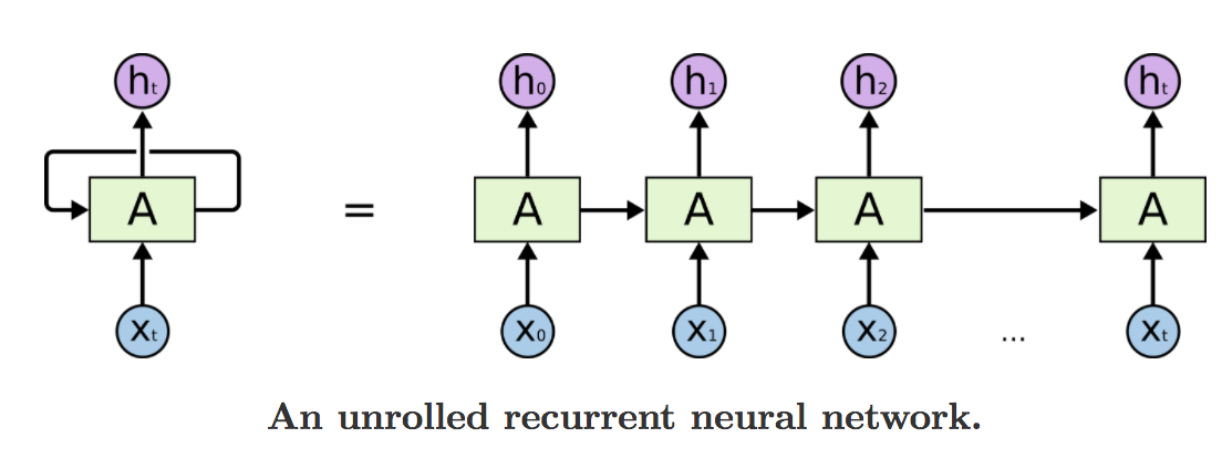
In the diagram above, a chunk of neural network (our RNN layer) takes some input $x_t$ and outputs a value $h_t$. This loop denotes the network will be repeating the process for every sequence in out input. In other words, when given a sentence of 4 words, the network (the RNN cell) will unrolled itself into 4 copies, one copy for each word.
The main issue with these vanilla RNN is that they tend to suffer from the vanishing gradient problem. Training a RNN is similar to training a traditional Neural Network, we also use the backpropagation algorithm, but with a little twist. Because the parameters are shared by all time steps in the network, the gradient at each output depends not only on the calculations of the current time step, but also the previous time steps. For example, in order to calculate the gradient at t=4 we would need to backpropagate 3 steps and sum up the gradients. This is called Backpropagation Through Time (BPTT). Thus we can imagine when computing the gradient, if we multiply a small number with another small number with another and with another, the value dramatically decays to 0, and the weights will no longer be updated when the gradients are 0. To mitigate this issue, other variants of RNNs were developed, and this notebook will look at one of them called LSTM (Long Short Term Memory).
LSTM Step by Step Walk Through
Note that a large portion of the content for this section is based on Blog: Understanding LSTM Networks
Given $x_t$, the input at time step $t$ and $h_t$, the hidden state at time step $t$ the computation happening in a vanilla RNN cell are as follow:
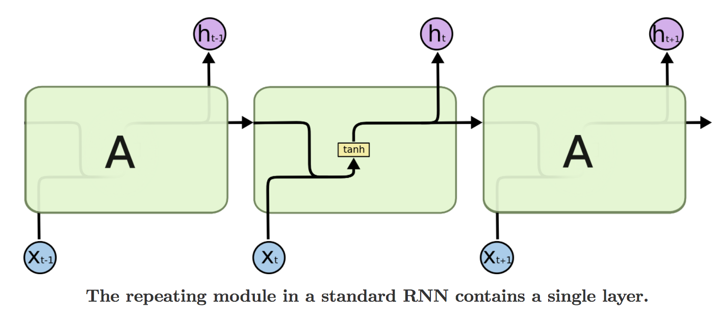
Here, $f$ is usually a nonlinearity function such as tanh. LSTMs also have this chain like structure, but the repeating module has a different structure. Instead of having a single set of weights $U$ and $W$ connecting the input and hidden state respectively, there are four sets of weights, interacting in a very special way.
LSTM are designed to avoid long-term dependency problems, and the core idea is the cell state, the horizontal line running through the top of the diagram.
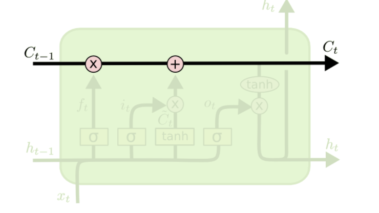
Cell state is kind of like a conveyor belt. It runs straight down the entire chain, with only some linear interactions, making it easier for information to flow along it unchanged. LSTMs have the ability to remove or add information to the cell state, carefully regulated by structures called gates. Namely, the forget gate, input gate and output gate.
The first step for a LSTM cell is to decide what information we're going to throw away from the cell state. This is determined by the a sigmoid layer "forget gate", the forget gate looks at $h_{t−1}$ and $x_t$, and outputs a number between 0 and 1 for each number in the cell state $C_{t−1}$. A 1 represents completely keep this while a 0 represents completely get rid of this.
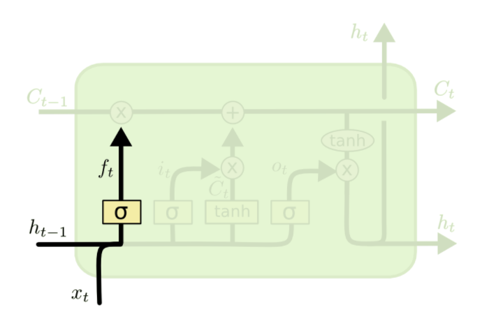
Note that $W_f \cdot [ h_{t - 1}, x_t ]$ is a simplified notation for $W h_{t - 1} + U x_t$, $W_f$ denotes that these are the set of weights for the forget gate.
For example, if we are building a language model that's trying to predict the next word based on all the previous ones. In such a problem, the cell state might include the gender of the present subject, to determine the correct pronouns to use. When we see a new subject, we want to forget the gender of the old subject.
The second step is to determine what new information to store in the cell state. This step consists of two parts, first a sigmoid layer known as the "input gate" decides which value we'll update. Second, a tanh layer creates a vector of new candidate value $\tilde{C_t}$, that could be added to the state.
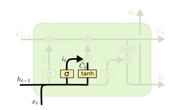
In the example of our language model, we want to add the gender of the new subject to the cell state to replace the old one we're forgetting.
It's now time to update the old cell state, $C_{t−1}$, into the new cell state $C_t$. The previous steps already decided what to do, we just need to actually do it. We multiply the old state by $f_t$, forgetting the things we've decided to forget earlier. Then we add $i_t * \tilde{C_t}$, which is the new cell state scaled by how much we've decided to update each value.
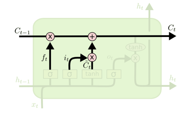
Looking at this formula more carefully, we can see that the information carried by the previous cell state, $C_{t-1}$ will not be lost if its weight, i.e. the forget gate $f_t$ is on (close to 1), making LSTM better at learning long-term dependencies compared to vanilla RNN.
In the case of the language model, this is where we'd actually drop the information about the old subject's gender and add the new information, as we decided in the previous steps.
Finally, we need to decide what we're going to output. This output will be a filtered version of our cell state. First, we run it through a sigmoid layer which decides what parts of the cell state we're going to output. This is essentially our output gate. Then, we put the cell state through tanh (to push the values to be between −1 and 1) and multiply it by the output of the sigmoid gate, so that we only output the parts we decided to.
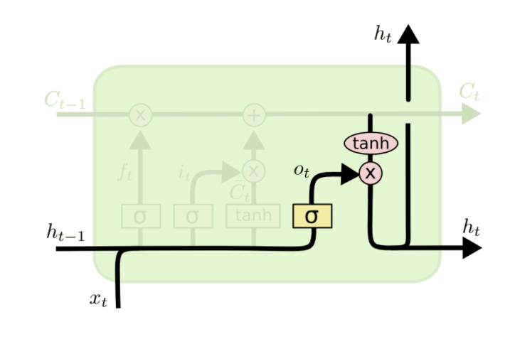
For the language model example, since it just saw a subject, it might want to output information relevant to a verb, in case that's what is coming next. Or it might output whether the subject is singular or plural, so that we know what form a verb the next word should take form.
Implementation
A lot of the scripts is similar to that of the implementation for vanilla RNN.
(X_train, Y_train), (X_test, Y_test) = mnist.load_data()
X_train = X_train.astype('float32')
X_test = X_test.astype('float32')

# images takes values between 0 - 255, we can normalize it
# by dividing every number by 255
X_train /= 255
X_test /= 255

print('mnist data shape: ', X_train.shape)
from dataloader import DataLoader


# Define some parameters
element_size = 28
time_steps = 28
num_classes = 10
batch_size = 128
hidden_layer_size = 128

# example of generating a batch of data using the
# DataLoader class
data_loader = DataLoader(X_train, Y_train, num_classes)
X_batch, y_batch = data_loader.next_batch(batch_size)
print('label shape: ', y_batch.shape)
print('data shape: ', X_batch.shape)
The formulas for LSTM is listed again for quick reference, note that for the implementation, we've excluded the bias term to keep things simpler.
\begin{align} f_t &= \sigma(W_f \cdot [ h_{t - 1}, x_t ] + b_f) \nonumber \\ i_t &= \sigma(W_i \cdot [ h_{t - 1}, x_t ] + b_i) \nonumber \\ \tilde{C_t} &= tanh(W_c \cdot [ h_{t - 1}, x_t ] + b_c) \nonumber \\ C_t &= f_t * C_{t-1} + i_t * \tilde{C_t} \nonumber \\ o_t &= \sigma(W_o \cdot [ h_{t - 1}, x_t ] + b_o) \nonumber \\ h_t &= o_t * tanh(C_t) \end{align}# the first dimension holds the batch size
inputs = tf.placeholder(tf.float32, shape = [None, time_steps, element_size], name = 'inputs')
labels = tf.placeholder(tf.float32, shape = [None, num_classes], name = 'labels')
# U : input's weight
# W : hidden state's weight
# the first dimension is 4 since we have 4 sets of these weights,
# 1 for forget gate, 1 for input gate, 1 for candidate cell state
# and 1 for output gate. We'll create them in 1 place and slice
# it to access each one
U = tf.Variable(tf.zeros([4, element_size, hidden_layer_size]))
W = tf.Variable(tf.zeros([4, hidden_layer_size, hidden_layer_size]))
def lstm_step(previous_hidden_state, x):
# lstm contains 2 sets of hidden state weights, 1 for the cell state
# and the other for the output state (originally the hidden state for
# vanilla RNN)
output_state, cell_state = tf.unstack(previous_hidden_state)
input_gate = tf.sigmoid(tf.matmul(x, U[0]) + tf.matmul(output_state, W[0]))
forget_gate = tf.sigmoid(tf.matmul(x, U[1]) + tf.matmul(output_state, W[1]))
output_gate = tf.sigmoid(tf.matmul(x, U[2]) + tf.matmul(output_state, W[2]))
candidate_cell_state = tf.tanh(tf.matmul(x, U[3]) + tf.matmul(output_state, W[3]))
new_cell_state = forget_gate * cell_state + input_gate * candidate_cell_state
new_output_state = output_gate * tf.tanh(new_cell_state)
current_hidden_state = tf.stack([new_output_state, new_cell_state])
return current_hidden_state
# the original input batch's shape is of [batch_size, time_steps and element_size]
# we permutate the order to [time_steps, batch_size, element_size]. The time_steps
# is put up front in order to leverage tf.scan's functionality
input_reshaped = tf.transpose(inputs, perm = [1, 0, 2])

# we initialize a hidden state to begin with and apply the rnn steps using tf.scan,
# which repeatedly applies a callable to our inputs
initial_hidden = tf.zeros([2, batch_size, hidden_layer_size])
all_hidden_states = tf.scan(
    lstm_step, input_reshaped, initializer = initial_hidden, name = 'hidden_states')

# if we do a fake run, we can see that the output at this point is the hidden state
# for every time step [time_steps, 2, batch_size, hidden_layer_size]
# 2 is for the 2 sets of hidden state LSTM has
with tf.Session() as sess:
    sess.run(tf.global_variables_initializer())

    data_loader = DataLoader(X_train, Y_train, num_classes)
    X_batch, y_batch = data_loader.next_batch(batch_size)
    temp = sess.run(all_hidden_states, feed_dict = {inputs: X_batch, labels: y_batch})
    print(temp.shape)
# output linear layer's weight and bias, V from the diagram
Wl = tf.Variable(tf.truncated_normal(
    [hidden_layer_size, num_classes],
    mean = 0, stddev = .01))
bl = tf.Variable(tf.truncated_normal(
    [num_classes], mean = 0,stddev = .01))

# apply linear layer to state vector;
# instead of calculating the output vector for every hidden state,
# in basic classification, we can assume the last hidden state
# has accumulated the information representing the entire sequence
states = tf.reshape(all_hidden_states[-1, 0], [-1, hidden_layer_size])
output = tf.matmul(states, Wl) + bl
learning_rate = 0.001

# specify the cross entropy loss, the optimizer to train the loss,
# the accuracy measurement
cross_entropy = tf.reduce_mean(
    tf.nn.softmax_cross_entropy_with_logits_v2(
    logits = output, labels = labels))
train_step = tf.train.RMSPropOptimizer(learning_rate).minimize(cross_entropy)
correct_prediction = tf.equal(tf.argmax(labels, axis = 1), tf.argmax(output, axis = 1))
accuracy = tf.reduce_mean(tf.cast(correct_prediction, tf.float32)) * 100
X_test_batch = X_test[:batch_size]
y_test_batch = to_categorical(Y_test[:batch_size], num_classes)

data_loader = DataLoader(X_train, Y_train, num_classes)

epochs = 5000
with tf.Session() as sess:
    sess.run(tf.global_variables_initializer())

    start = time()
    for i in range(epochs):
        X_batch, y_batch = data_loader.next_batch(batch_size)
        sess.run(train_step, feed_dict = {inputs: X_batch, labels: y_batch})

        if i % 1000 == 0:
            acc, loss = sess.run([accuracy, cross_entropy],
                                 feed_dict = {inputs: X_batch, labels: y_batch})
            print("Iter " + str(i) + ", Minibatch Loss =",
                  "{:.5f}".format(loss) + ", Training Accuracy =",
                  "{:.4f}".format(acc))

    print('Optimization finished!')
    acc_test = sess.run(accuracy, feed_dict = {inputs: X_test_batch, labels: y_test_batch})
    print('Test Accuracy: ', acc_test)
    print('elapse time: ', time() - start)
Conclusion
Given the more complex structure, it makes sense that it takes longer for LSTMs to train compared to vanilla RNN. But, thankfully, it does give better performance on the test set.
Most of exciting result today achieved by RNN-like networks is in fact achieved by LSTMs, because of its capability to deal with long term dependency. The long term dependency problem is that, when we have larger network through time, the gradient decays quickly during back propagation. So training a RNN having long unfolding in time becomes impossible. But LSTM avoids this decay of gradient problem by allowing us to make a super highway (cell states) through time, these highways allow the gradient to freely flow backward in time making them less susceptible to vanishing gradients.