%load_ext watermark

%watermark -a 'Ethen' -d -u

Author: Ethen

Last updated: 2023-07-03

Training Bi-Encoder Models with Contrastive Learning Notes¶

From a practical stand point, sentence embeddings are particular useful in:

Retrieval tasks where the typical setup is a bi-encoder, a.k.a. twin tower architecture model. These architecture accepts individual entity as inputs, and comparing them with future inputs for retrieving "similar" entities (definition of similar is use case dependent). This enables pre-computing embeddings and caching for retrieving "similar" entities through fast approximate nearest neighborhood look ups which is critical for latency sensitive applications.
Embedding-based classification tasks, where embeddings are fed in as features to downstream models. This is different from a typical fine-tuning setup, as these embeddings, once generated are considered frozen, and won't be tuned along with rest of our models. These are places where downstream application relies on non-deep learning models such as gradient boosted tree as their choice of machine learning algorithm.

Key Recipes¶

In this transformer-based deep learning era, it is often beneficial to warm start our models from pre-trained checkpoints. One important caveat is popular pre-trained models trained using masked language modeling objective such as BERT [16] or RoBERTA [17] doesn't generate meaningful sentence embeddings as per one of the original authors. SBERT (Sentence Bert) [5] further demonstrated it is beneficial to perform additional fine-tuning on top of pre-trained transformer based language models for competitive sentence embedding performance.

For fine-tuning procedure, many works including the original SBERT relied on classification, regression, pairwise triplet/hinge loss style objective function [5] [14] [15]. But one of SBERT authors later pointed out that contrastive learning is a much better approach [1] and E5 (EmbEddings from bidirEctional Encoder rEpresentations) [13] which also involves pre-training stage with contrastive learning tops the retrieval benchmark suite from MTEB (Massive Text Embedding Benchmark) [10]. So here we are, discussing some recipes for training sentence embeddings via contrastive learning.

As with most other use cases, we can of course use a more powerful encoder to generate the embedding representations for our input examples, but some tips specific to improve the performance for contrastive loss based learning involves:

Noise Contrastive Objective Function¶

In recent years, most contrastive learning procedures leverage variants of InfoNCE (Noise Contrastive Estimation) loss [11]. This type of loss, sometimes referred to as NT-Xent (normalized temperature scaled cross entropy loss) in as SimCLR (simple contrastive learning of visual representations) [12] or multiple negative ranking loss [2], uses cross entropy loss to distinguish positive from potentially multiple negative examples.

\begin{aligned} \mathcal{L} = & -\log \frac{\exp \left(\operatorname{sim}\left(\boldsymbol{a}_i, \boldsymbol{p}_i\right) / \tau\right)}{\exp \left(\operatorname{sim}\left(\boldsymbol{a}_i, \boldsymbol{p}_i\right) / \tau\right) + \sum_{j=1}^m \exp \left(\operatorname{sim}\left(\boldsymbol{a}_i, \boldsymbol{n}_j\right) / \tau\right)} \end{aligned}

For training this loss function, we need to have pairs of anchors and its corresponding positive example. Here:

$a_i$, $p_i$ denotes embedding respresentation of our anchor and positive examples. What we wish to accomplish is $a_i$ and $p_i$ becoming close in the vector space, whereas $a_i$ and other $m$ negative examples $n_j$ becomes distant apart. We'll discuss how negative examples can be derived in up coming paragraphs.
$sim$ here represents a similarity function such as cosine similarity or dot product.
$\tau$ denotes temperature scaling which can be a learned parameter, or configurable value.

Note if choosing cosine similarity as similarity function, and $\tau$ is chosen by hand, we might need to lean towards a smaller value. As by default, cosine similarity's score differences are too small and doesn't lead to good empirical results.

CLIP (Contrastive Language-Image Pre-Training) [8] introduces a symmetric version of this loss function. PyTorch style pseudocode is shown below:

# @ denotes matrix multiplication, and represents a in batch negative
# operation mentioned in the next section.
scores = anchor_embedding @ positive_embedding.T / temperature
labels = torch.arange(len(scores), device=scores.device, dtype=torch.long)
cross_entropy_loss(scores, labels)

# clip style symmetric version
anchor_scores = anchor_embedding @ positive_embedding.T / temperature
positive_scores = positive_embedding @ anchor_embedding.T / temperature
labels = torch.arange(len(anchor_scores), device=scores.device, dtype=torch.long)
loss = (cross_entropy_loss(anchor_scores, labels) + cross_entropy_loss(positive_scores, labels)) / 2

anchor_embedding and positive_embedding are embedding representation of anchor and positive samples, in the shape of [batch size, hidden size]. They are generated by backbone encoder (e.g. transformer) with or without linear projection of our choice. The encoder can even share weights, which is commonly referred to as siamese network.

Large In Batch Negatives¶

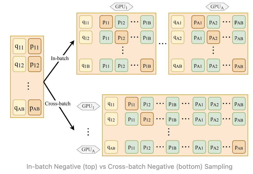
In batch negatives is widely used for training models with contrastive loss. Assuming there are $B$ positive pairs for a given mini batch, each of these positive pairs can be paired with $B - 1$ negatives (rest of the positive pairs within the same mini batch). This paradigm allows us to leverage the already loaded mini batch rather than using additional resources to sample negative examples. When relying on in batch negative sampling, using a larger batch size is key, as it allows the loss function to optimize over a more diverse set of negative samples. i.e. it's easier to find the right answer over a pool of 2 candidates, versus say 1024 candidates. This can be treated as an implicit version of hard negative mining.

Work such as RocketQA [6] and CLIP [8] further mentions the use of cross gpu/batch negatives, where when training on multiple GPUs, the embedding calculation can be sharded within each single GPU, these embeddings can then be shared among all GPUs and serves as additional negative examples. i.e. for A GPUs, we can now collect $A \times B - 1$ negatives. Note, sharing here refers to a differentiable all gather operation.

With this approach, CLIP reports to be using a effective batch size as large as 32,768 sharded across 256 GPUs, it should be noted that the optimal size will be dependent on training data size, where CLIP's training data consists of more than 400M examples. As with all hyper parameters, the optimal setting will be use-case dependent. When pressed for time, this is most likely the parameter that we should prioritize on tuning above everything else.

Given the importance of large batch size in contrastive learning, it can be helpful to employ techniques that:

Reduces memory consumption during training so we can safely enlarge our micro batch size without resulting in out of memory issues when training large scale models. This includes:
- Deepspeed's zero optimization stage 2 [28], which removes the memory redundancies across data-parallel processes by partitioning optimizer states as well as gradients across nodes.
- Gradient/Activation checkpointing. In order to compute gradients during backward pass, all activations from the forward pass are normally saved. Gradient checkpointing saves strategically selected activations throughout the computational graph and recompute them on demand during backward pass.
Design a curriculum learning [37] style training procedure, where we gradually increase contrastive learning's effective batch size.

Mine Hard Negatives¶

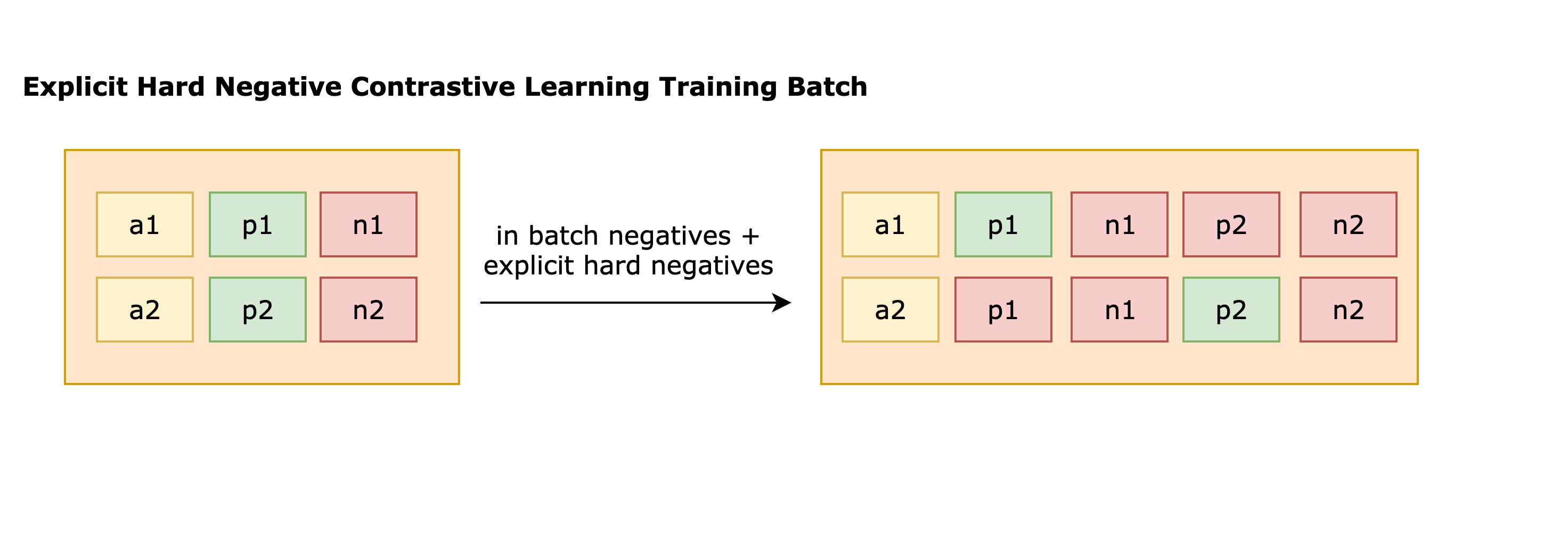
By increasing training batch size for our in-batch negative sampling, we can generate a larger number of negative samples from in batch negative sampling. However, many of these negatives may be easily distinguishable by our model, thereby providing limited additional information after a certain point. To address this, we need a mechanism to identify hard negatives, which are more challenging for the model to discern. In other words, instead of providing pairs of anchors, $a_i$, and positives, $p_i$ as our input data. We now provide triplets $a_i, p_i, n_i$, where negative $n_i$ should be similar to $p_i$ but shouldn't match with $a_i$. While forming a contrastive learning training batch, these explicit hard negatives will be concatenated along with other in batch negatives as shown in the diagram below.

It is worth noting:

Negative can be an array of negatives and not just a single instance.
This supposedly also alleviate selection bias, giving the model better resolution towards samples that are not in our positive examples set [30].
Adding these hard negatives doesn't change our InfoNCE style contrastive learning loss, the only difference being now our $m$ negative examples, $n_j$ includes both in batch negatives as well as these additionally mined explicit hard negatives.

Primary strategies of providing these hard negatives includes:

Leveraging structure from our data [1], this strategy relies on our creativity and domain knowledge. For example:
- For stackexchange question and answering dataset that contains sub-forums talking about programming, travel, cooking, creating pairs from each sub-forums while likely yield higher quality batches.
- Or let's say we have a paper citation dataset, given a seed paper representing our anchor example, we can use the seed paper's cited paper as positive, while the paper that is cited by our cited paper, but not cited by the seed paper acting as negatives.
- If we are working with website logs, using users engagement such as impressions, clicks or purchases [15] [29]. e.g. For a stackoverflow question and answering dataset, we can take answers with many upvotes and the positive sample and answers without any upvotes as hard negatives.
Algorithmically generate them.
- RocketQA [6], Augmented SBERT [7], DPR (Dense Passage Retrieval) [9] suggests mining hard negatives using BM25 or a trained bi-encoder to generate semantically similar hard negatives. These model dependent methods are likely to perform better than performing lexical edits like insert/swap/delete/synonym replace [4]. ANCE (Approximate nearest neighbor Negative Contrastive Estimation) [32] even proposes using an asynchronously updated ANN index to continuously mine hard negatives from a trained bi-encoder throughout the training process
- For images, there're plethora of image augmentation techniques, e.g. random cropping, resize, color distortion, gaussian blur, etc. All are methods to transform pixels while preserving the semantic meaning of an image's content such as its class labels. In un-supervised context such as SimCLR [12], where they rely on data augmentations to create positive pairs, they argue that stronger data augmentation is needed for contrastive learning to learn strong representations compared to the supervised counterparts, where the composite augmentation random cropping and color distortion was shown to stand out.

With this strategy, we need to be mindful and ensure these examples are actually negatives. It is typically infeasible to scan through our entire dataset and label all the positive examples for a given anchor. Hence it can happen when sampling hard negatives, we might accidentally sample a positive example that wasn't labeled, introducing false negatives to the mix. To solve for this, we can train a separate cross-encoder model, which are typically more powerful at capturing semantic similarity compared to bi-encoder to denoise our hard negatives. In other words, when sampling hard negatives from the top ranked examples using aforementioned strategies, we can only select the ones that are predicted as negatives by the cross encoder with high confidence score.

Training with a mix of both random, hard negatives is often times beneficial, what's the optimal proportion of the two is something we'll have to experiment with on our use case. The overall data augmentation workflow can be roughly summarized into the following steps [6] [7]:

First train both a bi-encoder and cross-encoder model.
We select additional input pairs and use our cross-encoder to label new input pairs, i.e. generate soft labels. Selecting suitable pairs is crucial for this augmentation strategy's success, and simply combining random pairs may lead to suboptimal downstream performance.
These additional pairs are added to the training set.
Fine-tune a new bi-encoder model on this larger augmented training dataset.
Rinse and repeat.

Data Augmentation¶

BEIR (Benchmarking Information Retrieval) [20] showed these dense embedding retrieval models require large amounts of training data to work well. If we are lacking data for a particular domain of interest, one trend in informational retrieval is to leverage generative models to generate synthetic data for training ranking models. At its core, the idea is large generative models have demonstrated impressive results across the board on many NLP tasks, however, they can be expensive to apply at run time. Hence, instead of using them directly in our system, we would like to apply them in an offline setting, where we use them to generate more in-domain training data for training our actual retrieval or ranking model. This arguably can be seen as an alternative form of distillation, where we aim to distill the knowledge of large generative models into small bi-encoder or cross encoder models via prompt generation. This high level workflow is depicted in the figure below:

To elaborate:

We randomly sample 100,000 documents from the collection, $D$ and generate one question, $q$ per document. In open sourced landscape, training on MS MARCO dataset was shown to provide reasonable out of domain performance. Caveat: the dataset's license prevents it from being used in a commerical context.
This generation process can be done via prompting a language or seq2seq model of choice (e.g. GPT-J) using only a few supervised examples.
From that collection of generated pairs, we pick the top K=10,000 pairs as positive examples for finetuning our models. This filtering step, sometimes referred to as consistency check can be done via training a bi-encoder model (e.g. from MiniLM, Deberta v3, etc.) on the generated pairs, then for each query, we retrieve a set of documents, and mark a query as passing the consistency check if the top-k retrieved document was the document from which the query was generated.
Given our re-ranker models are binary classifiers, we also need a way to select negative pairs, $(q, d−)$. This can be done via BM25 or from a trained bi-encoder, with $q$ as query to retrieve top documents from the collection $D$. We randomly select one of these as $d−$.

We can imagine many variations that can stem out of this workflow: including different prompting template as well as which language or seq2seq model to use, choice of re-ranker models etc. Work such as InPars (Inquisitive Parrots for Search) v1/v2/light [22] [23] [24], Prompt base Query Generation for Retriever (PROMPTAGATOR) [25], GPL (Generative Pseudo Labeling) [26] all demonstrates different design choices and its effectiveness to various degree.

Others¶

Note, in pure image field work such as Moco (Momentum Contrast) [18] introduces the concept of memory queue and momentum encoder for improving contrastive learning results. Both of them are not elaborated upon here as:

Memory queue was shown to be unnecessary when given large enough batch size in Moco v3 [19].
These techniques were applied to an unsupervised image setting, whereas text settings work such as E5 [13] claims training with bigger batch size is more stable and results in no performance difference.
Note that the underlying mechanism of momentum encoders will double our GPU memory consumption (since it requires keeping a copy of existing trainable models). This might not be very practical when we wish to scale up backbone encoder size for improving performance, unless we devote to introducing model parallel in our training infrastructure.

Public Dataset & Benchmark¶

We can refer to public pre-trained sentence transformer's model card [3], and E5 [13] on public datasets that can be combined and used to fine-tune these models .

As with all methods, it is important to find an established benchmark dataset so we can quickly iterate on new ideas. MTEB [10], has collected 8 embedding tasks ranging from semantic textual similarity (STS, SemEval), classification (fine tuning a classifier using the embedding as input features, SentEval), information retrieval (BEIR [20]), etc., in total it consists of 56 datasets, covering 112 languages. They also evaluated 30 different models to provide a holistic view of state of the art public pre-trained text embedding models.

Final Remarks¶

Two tower based models are extremely popular in industrial for various embedding based retrieval use case, and for good reasons:

Hybrid/Ensemble. They can complement existing token/keyword based retrieval systems [34].
Efficiency. In a common setup of retrieving items based on a particular context (common ones includes query or user), we can pre-compute and cache the item representation/embeddings. At inference time, we would only need to calculate a single embedding for our context, and perform an approximate nearest neighbor (ANN) search.
Alleviate cold start problem. Two tower based models often takes in additional metadata as input features instead of purely relying on user and item ids.

Non-exhaustive list of their presence in the industry includes: Amazon's semantic product search [14] as well as query rewrite [35], Facebook search's multi-modal embedding based retrieval [15] [29], Google play's retrieval system [30], Youtube's fresh content retrieval [36], Bing sponsored search's multi-objective retrieval system [31].

Even in the context of modern large language model, retrieval augmented generation [33] is still a highly efficient method to avoid stuffing everything inside a model's prompt, and having to fear the need to re-train this model to prevent generating potentially out-dated information.

References¶

[1] Youtube: Training State of the Art Sentence Embedding Models
[2] SBERT Documentation - Multiple Negatives Ranking Loss
[3] Model Card: sentence-transformers/all-MiniLM-L12-v2
[4] Github: Data augmentation for NLP
[5] Nils Reimers, Iryna Gurevych - Sentence-BERT: Sentence Embeddings using Siamese BERT-Networks - 2019
[6] Kai Liu, Ruiyang Ren, Wayne Xin Zhao, et al. - RocketQA: An Optimized Training Approach to Dense Passage Retrieval for Open-Domain Question Answering - 2021
[7] Nandan Thakur, Nils Reimers, Johannes Daxenberger, Iryna Gurevych - Augmented SBERT: Data Augmentation Method for Improving Bi-Encoders for Pairwise Sentence Scoring Tasks - 2020
[8] Alec Radford, Jong Wook Kim, et. al - Learning Transferable Visual Models From Natural Language Supervision - 2021
[9] Vladimir Karpukhin, Barlas Oğuz, et al. - Dense Passage Retrieval for Open Domain Question Answering - 2020
[10] Niklas Muennighoff, Nouamane Tazi, Loïc Magne, Nils Reimers - MTEB: Massive Text Embedding Benchmark - 2022
[11] Aaron van den Oord, Yazhe Li, Oriol Vinyals - Representation Learning with Contrastive Predictive Coding - 2018
[12] Ting Chen, Simon Kornblith, Mohammad Norouzi, Geoffrey Hinton - A Simple Framework for Contrastive Learning of Visual Representations - 2020
[13] Liang Wang, Nan Yang, Xiaolong Huang, Binxing Jiao, Linjun Yang, Daxin Jiang, Rangan Majumder, Furu Wei - Text Embeddings by Weakly-Supervised Contrastive Pre-training - 2022
[14] Priyanka Nigam, Yiwei Song, etc. - Semantic Product Search - 2019
[15] Jui-Ting Huang, Ashish Sharma, Shuying Sun, Li Xia, David Zhang, Philip Pronin, Janani Padmanabhan, Giuseppe Ottaviano, Linjun Yang - Embedding-based Retrieval in Facebook Search - 2020
[16] Jacob Devlin, Ming-Wei Chang, Kenton Lee, Kristina Toutanova - BERT: Pre-training of Deep Bidirectional Transformers for Language Understanding - 2018
[17] Yinhan Liu, Myle Ott, Naman Goyal, Jingfei Du, etc. - RoBERTa: A Robustly Optimized BERT Pretraining Approach - 2019
[18] Kaiming He, Haoqi Fan, Yuxin Wu, Saining Xie, Ross Girshick - Momentum Contrast for Unsupervised Visual Representation Learning - 2019
[19] Xinlei Chen, Saining Xie, et al. - An Empirical Study of Training Self-Supervised Vision Transformers - 2021
[20] Nandan Thakur, Nils Reimers, Andreas Rücklé , Abhishek Srivastava, Iryna Gurevych - BEIR: A Heterogeneous Benchmark for Zero-shot Evaluation of Information Retrieval Models - 2021
[21] Vespa Blog: Improving Search Ranking with Few-Shot Prompting of LLMs
[22] Luiz Bonifacio, Hugo Abonizio, Marzieh Fadaee, Rodrigo Nogueira - InPars: Data Augmentation for Information Retrieval using Large Language Models - 2022
[23] Vitor Jeronymo, Luiz Bonifacio, Hugo Abonizio, Marzieh Fadaee, Roberto Lotufo, Jakub Zavrel, Rodrigo Nogueira - InPars-v2: Large Language Models as Efficient Dataset Generators for Information Retrieval - 2023
[24] Leonid Boytsov, Preksha Patel, Vivek Sourabh, Riddhi Nisar, Sayani Kundu, Ramya Ramanathan, et al. - InPars-Light: Cost-Effective Unsupervised Training of Efficient Rankers - 2023
[25] Zhuyun Dai, Vincent Y. Zhao, Ji Ma, Yi Luan, et al. - Promptagator: Few-shot Dense Retrieval From 8 Examples - 2022
[26] Kexin Wang, Nandan Thakur, Nils Reimers, Iryna Gurevych - GPL: Generative Pseudo Labeling for Unsupervised Domain Adaptation of Dense Retrieval - 2021
[27] Blog: Positive and Negative Sampling Strategies for Representation Learning in Semantic Search
[28] Samyam Rajbhandari, Jeff Rasley, et al. - ZeRO: Memory Optimizations Toward Training Trillion Parameter Models - 2019
[29] Yunzhong He, Yuxin Tian, et al. - Que2Engage: Embedding-based Retrieval for Relevant and Engaging Products at Facebook Marketplace - 2023
[30] Ji Yang, Xinyang Yi, Derek Zhiyuan Cheng, Lichan Hong, Yang Li, Simon Wang, Taibai Xu, and Ed H. Chi - Mixed Negative Sampling for Learning Two-tower Neural Networks in Recommendations - 2020
[31] Jianjin Zhang, Zheng Liu, Weihao Han, Shitao Xiao, Ruicheng Zheng, Yingxia Shao, Hao Sun, Hanqing Zhu, Premkumar Srinivasan, Denvy Deng, Qi Zhang, Xing Xie - Uni-Retriever: Towards Learning The Unified Embedding Based Retriever in Bing Sponsored Search - 2022
[32] Lee Xiong, Chenyan Xiong, et al. - Approximate Nearest Neighbor Negative Contrastive Learning for Dense Text Retrieval - 2020
[33] Blog: Knowledge Retrieval Architecture for LLM’s (2023)
[34] Blog: Beware Tunnel Vision in AI Retrieval
[35] Yupin Huang, Jiri Gesi, Xinyu Hong, Han Cheng, Kai Zhong, Vivek Mittal, Qingjun Cui, and Vamsi Salaka - Behavior-driven Query Similarity Prediction based on Pre-trained Language Models for E-Commerce Search - 2023
[36] Jianling Wang, Haokai Lu, et al. - Fresh Content Needs More Attention: Multi-funnel Fresh Content Recommendation - 2023
[37] Yoshua Bengio, Jerome Louradour, Ronan Collobert, Jason Weston - Curriculum Learning - 2009