os.chdir(path)

# 1. magic for inline plot
# 2. magic to print version
# 3. magic so that the notebook will reload external python modules
%matplotlib inline
%load_ext watermark
%load_ext autoreload 
%autoreload 2

import numpy as np
import pandas as pd
import tensorflow as tf

%watermark -a 'Ethen' -d -t -v -p numpy,pandas,tensorflow

Ethen 2017-03-20 13:44:55 

CPython 3.5.2
IPython 4.2.0

numpy 1.12.0
pandas 0.19.2
tensorflow 1.0.1

Convolutional Networks¶

When we hear about Convolutional Neural Network (CNN or ConvNet), we typically think of Computer Vision. CNNs were responsible for major breakthroughs in Image Classification and are the core of most Computer Vision systems today, from Facebook’s automated photo tagging to self-driving cars.

Motivation¶

Convolutional Neural Networks (ConvNet) are very similar to ordinary neural networks. They are made up of neurons that have learnable weights and biases. Each neuron receives some inputs, performs a dot product with the weights and biases then follows it with a non-linearity. The whole network still expresses a single differentiable score function: from the raw image pixels on one end to class scores at the other. And they still have a loss function (e.g. SVM/Softmax) on the last (fully-connected) layer hence most of the tips/tricks we developed for learning regular Neural Networks still apply.

The thing is: Regular Neural Nets don't scale well to full images. For the CIFAR-10 image dataset, images are only of size 32, 32, 3 (32 wide, 32 high, 3 color channels), so a single fully-connected neuron in a first hidden layer of a regular Neural Network would have 32x32x3 = 3072 weights. This amount still seems manageable, but clearly this fully-connected structure does not scale to larger images. For example, an image of more respectable size, e.g. 200x200x3, would lead to neurons that have 200x200x3 = 120,000 weights. Moreover, we would almost certainly want to have several such neurons, so the parameters would add up quickly! Clearly, this full connectivity is wasteful and the huge number of parameters would quickly lead to overfitting.

Thus unlike a regular Neural Network, ConvNet architectures make the explicit assumption that the inputs are images, which allows us to encode certain properties into the architecture. These then make the forward function more efficient to implement and vastly reduce the amount of parameters in the network. More explicitly, the layers of a ConvNet have neurons arranged in 3 dimensions: width, height, depth. (Note that the word depth here refers to the third dimension of an activation volume, not the depth of a full Neural Network, which can refer to the total number of layers in a network.) For example, the input images in CIFAR-10 are input volumes of 32x32x3 (width, height, depth respectively).

We use three main types of layers to build ConvNet architectures: Convolutional Layer, Pooling Layer, and Fully-Connected Layer (exactly as seen in regular Neural Networks). We will stack these layers to form a full ConvNet architecture.

Convolutional Layer¶

The Conv layer is the core building block of a Convolutional Network that does most of the computational heavy lifting.

Convolutional Layer-1 Basics¶

Each layer can be visualized in the form of a block. For instance in the case of CIFAR-10 data, the input layer would have the following form:

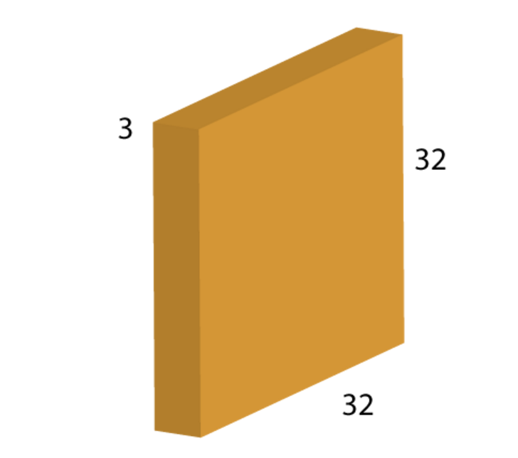
Here you can see, this is the original image which is 32×32 in height and width. The depth here is 3 which corresponds to the Red, Green and Blue (RGB) colors. A convolution layer is formed by convolving a filter or so called the kernel over it. A filter is another block that has a smaller height and width usually 3x3, 5x5 or somthing that like, but must has SAME depth size, which is swept over its input block. Let’s consider a filter of size 5x5x3 and see how it is done:

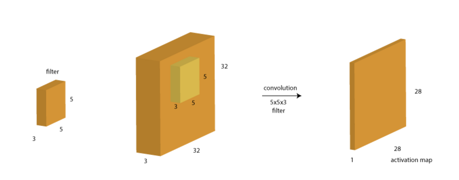
Convolving means that we take the filter and start sliding it over all possible spatial locations of the input from the top left corner to the bottom right corner. This filter is a set of weights, i.e. 5x5x3=75 + 1 bias = 76 weights in total (the filter weights are parameters which are learned during the backpropagation step). At each position, the weighted sum of the pixels is calculated as $W^TX + b$ and a new value is obtained.

After the computation for a single filter, we end up with a a volume of size 28x28x1 (more on this later) as shown above. This is often referred to as the activation map.

Another way of think of this process is that it is as a sliding window function. Consider the following gif:

Convolution with 3×3 Filter

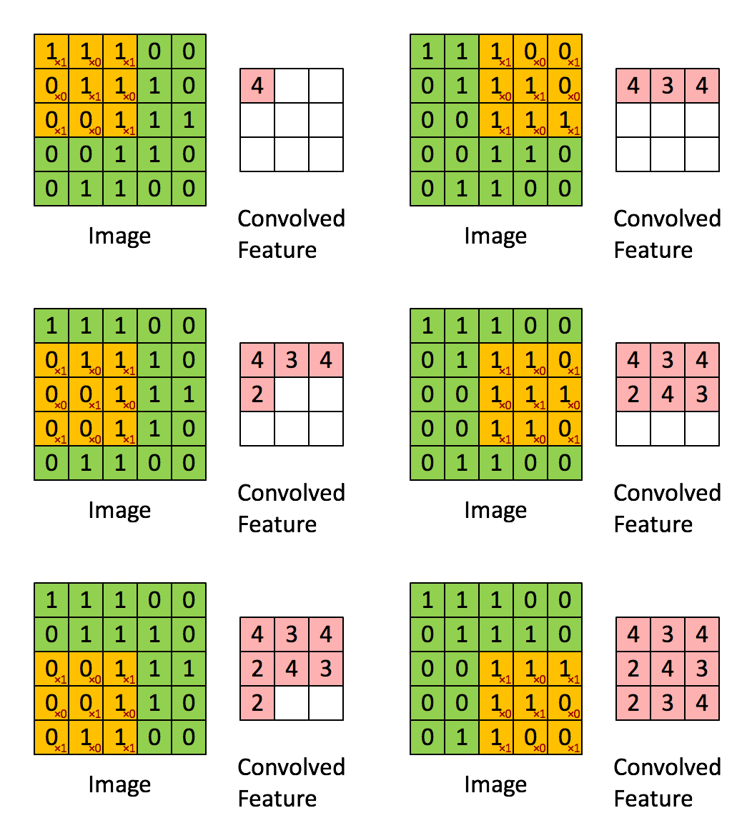
Imagine that the matrix on the left represents an black and white image. Each entry corresponds to one pixel, 0 for black and 1 for white (typically it’s between 0 and 255). Here we use a 3×3 filter, multiply its values element-wise with the original matrix, then sum them up. To get the full convolution we do this for each element by sliding the filter over the whole matrix.

For this step of the process, we usually want to have multiple filters (each independent of each other). Therefore, if 10 filters (the number is a hyperparameter that we can tune) are used, the output would look like:

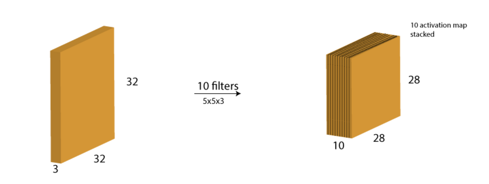
The result of the process is we've just represented the original image with a 28x28x10 activation maps that are stacked together along the depth dimension. And this activation map will be feed into later processing.

Convolutional Layer-2 Spatial Dimensions¶

You might have noticed that we got a block of size 28×28 as the output when the input was 32×32. Why so? Let’s look at a simpler case. Suppose the initial image has a of size 6x6xd and the filter takes a size of 3x3xd. Since depth size of the input and the filter is always same, we can only look at it from a top-down view (leaving out the depth) perspective.

Here we can see that the output will be 4x4xd volume block (4 distinct positions in one row and there're 4 rows in total).

Let's define a generic case where image has dimension $N \times N \times d$ and filter has $F \times F \times d$. Also, lets define another term stride (S) another hyperparameter, which is the number of cells (in the matrix above) to move in each step. We had a stride of 1 but it can be a higher value as well. Given these information the size of the output can be computed by the following formula:

$$(N – F)/S + 1$$

You can validate the formula with the example above or with the CIFAR-10 image dataset where $N=32$, $F=5$, $S=1$ where the output is 28.

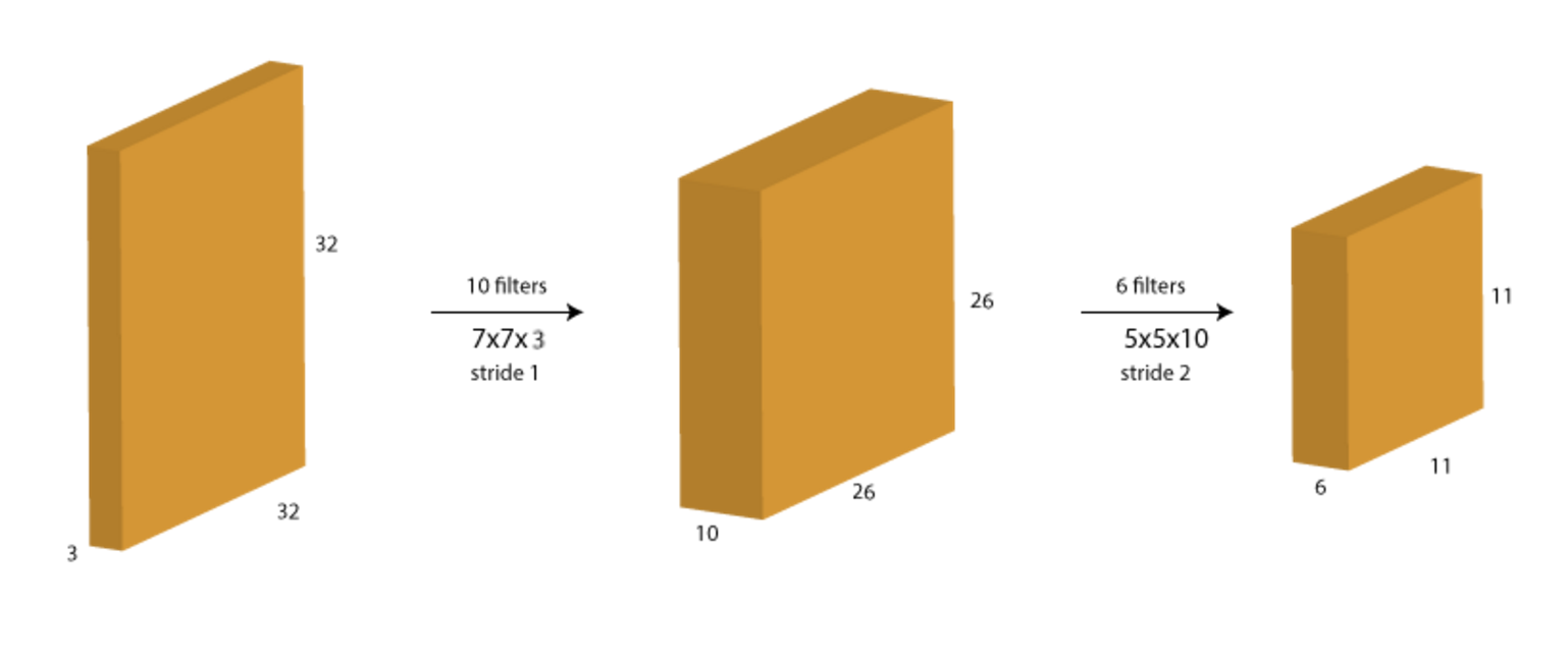
Note that some $S$ values might lead to non-integer result and we generally don't use such values, different libraries might deal with it different (e.g. throw an error).

Let's consider another example to consolidate our understanding. Starting with the same image as before of size 32×32, we apply 2 filters consecutively, first 10 filters of size 7, stride 1, next 6 filters of size 5, stride 2. Before looking at the solution below, just think about 2 things:

What should be the depth of each filter?
What will the resulting size of the images in each step?

Answer:

Notice in the second layer, the filters are now 5x5x**10** because **10** is the depth of its input.

Convolutional Layer-3 Paddings¶

Notice from the picture above, that the size of the input is shrinking consecutively (from 32 to 26 to 11). This will be undesirable in case of deep networks where the size will become very small too early and we'll loose a lot of representations of the original input. Also, it would restrict the use of large size filters as they would result in faster size reduction.

To prevent this, we generally use a stride of 1 along with zero-padding of size $(F-1)/2$. Zero-padding is nothing but adding additional zero-value pixels along every border of the image.

Consider the example we saw above with 6×6 image and 3×3 filter. The required padding is (3-1)/2=1. We can visualize the padding as:

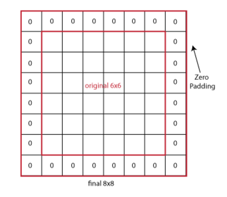
Here you can see that the image now becomes 8×8 because of padding of 1 on each side. So now by plugging in the number to the output size formula, $(N – F)/S + 1$, we will notice the output will be of size 6×6, ( 8 - 3 ) / 1 + 1 = 6, which is the same as the original input size.

Given this new information, we can write down the final formula for calculating the output size. The output width and height is a function of the input volume size (N), the filter size of the Conv Layer (F), the stride with which they are applied (S) and the amount of zero padding used (P) on the border:

$$(N−F+2P)/S+1$$

And the depth is simply the number of filters that we have.

Example: Input volumn of 32x32x3, what is the output size if we're to apply 10 5x5 filters with stride 1 and pad 2. And what is the total number of weights for this layer?

The output width and the height will be ( 32 - 5 + 2 * 2 ) / 1 + 1 = 32 and the depth will be 10.
The total number of weights will be the filter size times the depth plus one for the bias and mutiply that with the total number of filters ( 5 x 5 x 3 + 1 ) * 10 = 760.

This github repo, Github: Convolution arithmetic contains animations of different types of convolutional layers if you're interested.

Pooling Layer¶

Recall that we use padding in convolution layer to preserve input size. The pooling layers are used to REDUCE the size of input. They're in charge of downsampling the the network to make it more manageable. The most common form of performing the downsampling is by max-pooling.

Consider the following 4×4 layer. So if we use a 2×2 filter with stride 2 and max-pooling, we get the following response:

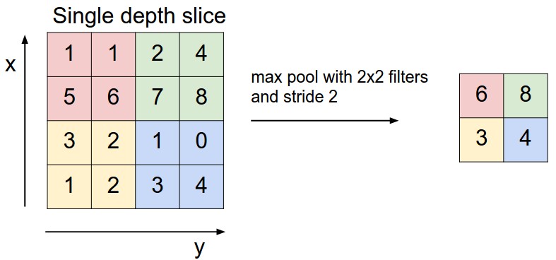
Here we can see that each 2×2 matrix are combined into 1 single number by taking their maximum value. Generally, max-pooling is used and works best but there're other options like average pooling.

It is common to periodically insert a pooling layer in-between successive Conv layers in a ConvNet architecture. Its function is to progressively reduce the spatial size of the representation to reduce the amount of parameters and computation in the network, and hence to also control overfitting.

The most common form is a pooling layer with filters of size 2x2 applied with a stride of 2. Every max-pooling operation would in this case be taking a max over 4 numbers (little 2x2 region in some depth slice). The depth size remains unchanged for this operation.

Summary of Conv and Pool Layer

The Conv Layer:

Accepts a volume of size $W_1 \times H_1 \times D_1$ (stands for width, height, depth)
Requires four hyperparameters:
- Number of filters $K$
- The filter's size $F$
- The stride $S$
- The amount of zero padding $P$
Produces a volume of size $W_2 \times H_2 \times D_2$ where:
- $W_2 = (W_1 - F + 2P)/S + 1$
- $H_2 = (H_1 - F + 2P)/S + 1$ (i.e. width and height are computed equally)
- $D_2 = K$
Each layer introduces $F \cdot F \cdot D_1$ weights per filter, for a total of $(F \cdot F \cdot D_1) \cdot K$ weights and $K$ biases.

Some common settings for these hyperparameters are $K = \text{ power of 2, e.g. 32, 64, 128, } F = 3, S = 1, P = 1$.

The Pooling Layer:

Accepts a volume of size $W_1 \times H_1 \times D_1$
Requires two hyperparameters:
- The filter's size $F$
- The stride $S$
Produces a volume of size $W_2 \times H_2 \times D_2$ where:
- $W_2 = (W_1 - F)/S + 1$
- $H_2 = (H_1 - F)/S + 1$
- $D_2 = D_1$
Introduces zero parameters since it computes a fixed function of the input
Note that it is not common to use zero-padding for Pooling layers

It is worth noting that there are only two commonly seen variations of the max pooling layer found in practice: A pooling layer with $F = 3, S = 2$ (also called overlapping pooling), and more commonly $F = 2, S = 2$. Pooling sizes with larger receptive fields are too destructive.

Fully Connected Layer¶

At the end of convolution and pooling layers, networks generally use fully-connected layers in which each pixel is considered as a separate neuron just like a regular neural network. The last fully-connected layer will contain as many neurons as the number of classes to be predicted. For instance, in CIFAR-10 case, the last fully-connected layer will have 10 neurons since we're aiming to predict 10 different classes.

Example ConvNet Architecture¶

Convolutional Networks are commonly made up of only three layer types: CONV, POOL (we assume Max pool unless stated otherwise) and FC (short for fully-connected). We will also explicitly write the RELU activation function as a layer, which applies element-wise non-linearity. In this section we discuss how these are commonly stacked together to form entire ConvNets.

The most common form of a ConvNet architecture stacks a few CONV-RELU layers, follows them with POOL layers, and repeats this pattern. At some point, it is common to transition to FC layers and the last fully-connected layer holds the output, such as the class scores (by applying softmax to it). In other words, the most common ConvNet architecture follows the pattern:

INPUT -> [ [CONV -> RELU] x N -> POOL?] x M -> [FC -> RELU] x K -> FC

where the x indicates repetition, and the POOL? indicates an optional pooling layer. Moreover, N >= 0 (and usually N <= 3), M >= 0, K >= 0 (and usually K < 3). For example, here are some common ConvNet architectures you may see that follow this pattern:

A simple ConvNet for CIFAR-10 classification could have the architecture [INPUT - CONV - RELU - POOL - FC]. In more detail:

INPUT layer [32x32x3] will hold the raw pixel values of the image, in this case an image of width 32, height 32, and with three color channels R,G,B.
CONV layer will compute the output of neurons that are connected to local regions in the input, each computing a dot product between their weights and a small region they are connected to in the input volume. This may result in volume such as [32x32x12] if we decided to use 12 filters.
RELU layer will apply an elementwise activation function, such as the $max(0,x)$ thresholding at zero. This leaves the size of the volume unchanged [32x32x12].
POOL layer will perform a downsampling operation along the spatial dimensions (width, height), resulting in volume such as [16x16x12].
FC (i.e. fully-connected) layer will compute the class scores, resulting in volume of size [1x1x10], where each of the 10 numbers correspond to a class score, such as among the 10 categories of CIFAR-10. As with ordinary Neural Networks and as the name implies, each neuron in this layer will be connected to all the numbers in the previous volume.

Course Note: Standford cs231n convolutional-networks contains a case study section at the bottom that introduces of different architectures.

Common Layer Sizing¶

The input layer (that contains the image) should be divisible by 2 many times. Common numbers include 32 (e.g. CIFAR-10), 64, 96 (e.g. STL-10), or 224 (e.g. common ImageNet ConvNets), 384, and 512. And images are squished to be rectangular shaped if they weren't already.

The conv layers should be using small filters (e.g. 3x3 or at most 5x5), using a stride of $S = 1$, and crucially, padding the input volume with zeros in such way that the conv layer does not alter the spatial dimensions of the input. That is, when $F = 3$, then using $P = 1$ will retain the original size of the input. When $F = 5$, $P = 2$. For a general $F$, it can be seen that $P = (F - 1) / 2$ preserves the input size. If you must use bigger filter sizes (such as 7x7 or so), it is only common to see this on the very first conv layer that is looking at the input image.

The pool layers are in charge of downsampling the spatial dimensions of the input. The most common setting is to use max-pooling with 2x2 receptive fields (i.e. filter size $(F) = 2$), and with a stride of 2 (i.e. $S = 2$). Note that this discards exactly 75% of the activations in an input volume (due to downsampling by 2 in both width and height). Another slightly less common setting is to use 3x3 receptive fields with a stride of 2. It is very uncommon to see receptive field sizes for max pooling that are larger than 3 because the pooling is then too lossy and aggressive. This usually leads to worse performance.

Getting rid of pooling. Many people dislike the pooling operation, since it loses information and think that we can get away without it (in favor of architecture that only consists of repeated CONV layers). To reduce the size of the representation it is suggested to use larger stride in CONV layer once in a while. Discarding pooling layers has also been found to be important in training good generative models and it seems likely that future architectures will feature very few to no pooling layers.

Reducing sizing headaches. The scheme presented above is pleasing because all the CONV layers preserve the spatial size of their input, while the POOL layers alone are in charge of down-sampling the volumes spatially. In an alternative scheme where we use strides greater than 1 or don't zero-pad the input in CONV layers, we would have to very carefully keep track of the input volumes throughout the CNN architecture and make sure that all strides and filters "work out", and that the ConvNet architecture is nicely and symmetrically wired.

Why use stride of 1 in CONV? Smaller strides work better in practice. Additionally, as already mentioned stride 1 allows us to leave all spatial down-sampling to the POOL layers, with the CONV layers only transforming the input volume depth-wise.

Why use padding? In addition to the aforementioned benefit of keeping the spatial sizes constant after CONV, doing this actually improves performance. If the CONV layers were to not zero-pad the inputs and only perform valid convolutions, then the size of the volumes would reduce by a small amount after each CONV, and the information at the borders would be "washed away" too quickly.

Compromising based on memory constraints. In some cases (especially early in the ConvNet architectures), the amount of memory can build up very quickly with the rules of thumb presented above. For example, filtering a 224x224x3 image with three 3x3 CONV layers with 64 filters each and padding 1 would create three activation volumes of size [224x224x64]. This amounts to a total of about 10 million activations, or 72MB of memory (per image, for both activations and gradients). Since GPUs are often bottlenecked by memory, it may be necessary to compromise. In practice, people prefer to make the compromise at only the first CONV layer of the network. For example, one compromise might be to use a first CONV layer with filter sizes of 7x7 and stride of 2 (as seen in a ZF net). As another example, an AlexNet uses filer sizes of 11x11 and stride of 4.

Tensorflow Implementation¶

We'll start by using the helper function to download the MNIST dataset. Here mnist is a variable that stores the training, validation, and testing sets as numpy arrays. It also provides a function for iterating through data minibatches, which we will use below.

from tensorflow.examples.tutorials.mnist import input_data
mnist = input_data.read_data_sets('MNIST_data', one_hot = True)

# access the training data (images) and labels
X_train, y_train = mnist.train.images, mnist.train.labels
X_test, y_test = mnist.test.images, mnist.test.labels
n_input = X_train.shape[1]  # MNIST data input (image's shape: 28*28)
n_class = y_train.shape[1]  # MNIST total classes (0-9 digits)
print(n_input, n_class)

Extracting MNIST_data/train-images-idx3-ubyte.gz
Extracting MNIST_data/train-labels-idx1-ubyte.gz
Extracting MNIST_data/t10k-images-idx3-ubyte.gz
Extracting MNIST_data/t10k-labels-idx1-ubyte.gz
784 10

We'll then create placeholder X and y to hold our input data and label. The None indicates that the number of input observation can be of any size.

To feed the data into the convolutional layer, we'll need to reshape X to a 4d tensor, with the second and third dimensions corresponding to image's width and height (MNIST is 28x28), and the final dimension corresponding to the number of color channels (since MNIST is a grey-scale image, so its a 1). The -1 is a placeholder that says "adjust as necessary to match the size needed". It's a way of making the code be independent of the input batch size.

X = tf.placeholder(tf.float32, shape = [None, n_input])
y = tf.placeholder(tf.float32, shape = [None, n_class])

# Input Layer
# Reshape X to 4-D tensor: [batch_size, width, height, channels]
# MNIST images are 28x28 pixels, and have 1 color channel
X_image = tf.reshape(X, [-1, 28, 28, 1])

To create CNN model, we're going to need to create a lot of weights and biases. One should generally initialize weights with a small amount of noise for symmetry breaking, and to prevent 0 gradients. Since we're using ReLU neurons, it is also good practice to initialize them with a slightly positive initial bias to avoid "dead neurons". Instead of doing this repeatedly while we build the model, let's create two handy functions to do it for us.

def weight_variable(shape):
    # truncated normal randomly output values from 
    # normal distribution, excect values whose magnitude is more than 2 standard
    # deviations from the mean are dropped and re-picked
    initial = tf.truncated_normal(shape, stddev = 0.1)
    return tf.Variable(initial)

def bias_variable(shape):
    initial = tf.constant(0.1, shape = shape)
    return tf.Variable(initial)

Next we define our convolutional and pooling layers: Our convolutions uses a stride of one and are zero padded. padding = 'SAME' means the size of output will be the same as the one we'll later specify. Our pooling is plain old max pooling over 2x2 blocks. To keep our code cleaner, let's also define these operations into functions.

Arguments Question on stackoverflow. Why is the first and last value for stride is always 1, or strides[0] = strides[3] = 1?

If input tensor has 4 dimensions: [batch, height, width, channel], then the convolution operates on a 2D window on the height, width dimensions. Hence the typical usage is to set the first value (batch) to 1, since you don't usually want to skip over examples in your batch, or you shouldn't have included them in the first place. And last value (channel) also to 1, since we usually don't want to skip inputs or perform the operation across multiples channels at the same time.

def conv2d(X, W):
    # X is our input data and W is the filters 
    return tf.nn.conv2d(X, W, strides = [1, 1, 1, 1], padding = 'SAME')

def maxpool2d(X):
    # we always use a 2 by 2 filter
    return tf.nn.max_pool(X, ksize = [1, 2, 2, 1],
                          strides = [1, 2, 2, 1], padding = 'SAME')

We can now implement our first layer. It will consist of a convolution layer, followed by max pooling layer. The convolutional will compute 32 features for each 5x5 patch (32 5x5 filters). Hence its weight tensor will have a shape of [5, 5, 1, 32]. The first two dimensions are the patch size, the next is the number of input channels, and the last number is the number of output channels. We will also have a bias vector with a component for each output channel.

We then convolve our input data X, add the bias, apply the ReLU activation function and max pool. In order to build a deep network, we stack several layers of this type. The second layer will have 64 features for each 5x5 patch.

# network layer parameter
n_conv_size = 5
n_conv1_num = 32
n_conv2_num = 64

# Convolutional Layer #1
# Computes 32 features using a 5x5 filter with ReLU activation.
# Padding is added to preserve width and height.
# Input Tensor Shape: [batch_size, 28, 28, 1]
# Output Tensor Shape: [batch_size, 28, 28, 32]
W_conv1 = weight_variable([n_conv_size, n_conv_size, 1, n_conv1_num])
b_conv1 = bias_variable([n_conv1_num])
h_conv1 = tf.nn.relu(conv2d(X_image, W_conv1) + b_conv1)

# First max pooling layer with a 2x2 filter and stride of 2
# Input Tensor Shape: [batch_size, 28, 28, 32]
# Output Tensor Shape: [batch_size, 14, 14, 32]
h_pool1 = maxpool2d(h_conv1)

# Convolutional Layer #2
# Computes 64 features using a 5x5 filter.
# Padding is added to preserve width and height.
# Input Tensor Shape: [batch_size, 14, 14, 32]
# Output Tensor Shape: [batch_size, 14, 14, 64];
# note that the input size of the second layer 
# must match the output size of the first
W_conv2 = weight_variable([n_conv_size, n_conv_size, n_conv1_num, n_conv2_num])
b_conv2 = bias_variable([n_conv2_num])
h_conv2 = tf.nn.relu(conv2d(h_pool1, W_conv2) + b_conv2)

# Pooling Layer #2
# Second max pooling layer with a 2x2 filter and stride of 2
# Input Tensor Shape: [batch_size, 14, 14, 64]
# Output Tensor Shape: [batch_size, 7, 7, 64]
h_pool2 = maxpool2d(h_conv2)

Now that the image size has been reduced to 7x7 (Try confirming that it is indeed 7x7 by plugging the max pool layer formula way above), we add a fully-connected layer with 1024 neurons. To do so, we need reshape (flatten) the tensor from the pooling layer into a batch of vectors, multiply by a weight matrix, add a bias, and apply a ReLU.

To reduce overfitting, we will apply dropout before the final softmax layer. We create a placeholder for the probability that a neuron's output is kept during dropout. This allows us to turn dropout on during training, and turn it off during testing (specify it to be a value of 1). TensorFlow's tf.nn.dropout automatically handles scaling neuron outputs in addition to masking them, so dropout works without any additional scaling. For this small convolutional network, performance is actually nearly identical with and without dropout, but it is often very effective at reducing overfitting when training very large neural networks.

# Flatten tensor into a batch of vectors
# Input Tensor Shape: [batch_size, 7, 7, 64]
# Output Tensor Shape: [batch_size, 7 * 7 * 64]
flatten_size = 7 * 7 * n_conv2_num
h_pool2_flat = tf.reshape(h_pool2, [-1, flatten_size])

# Dense Layer, a.k.a fully connected layer
# Densely connected layer with 1024 neurons
# Input Tensor Shape: [batch_size, 7 * 7 * 64]
# Output Tensor Shape: [batch_size, 1024]
fc_size = 1024
W_fc1 = weight_variable([flatten_size, fc_size])
b_fc1 = bias_variable([fc_size])
h_fc1 = tf.nn.relu( tf.matmul(h_pool2_flat, W_fc1) + b_fc1 )

# dropout
keep_prob  = tf.placeholder(tf.float32)
h_fc1_drop = tf.nn.dropout(h_fc1, keep_prob)

# the final output layer
W_fc2 = weight_variable([fc_size, n_class])
b_fc2 = bias_variable([n_class])

# output
y_conv = tf.matmul(h_fc1_drop, W_fc2) + b_fc2

# network global parameter
learning_rate = 1e-4
dropout = 0.5
iteration = 5000
batch_size = 50

# specify the cross entropy loss, the optimizer to train the loss,
# the accuracy measurement and the variable initializer
cost = tf.reduce_mean(tf.nn.softmax_cross_entropy_with_logits(logits = y_conv, labels = y))
train_step = tf.train.AdamOptimizer(learning_rate).minimize(cost)
correct_prediction = tf.equal( tf.argmax(y_conv, axis = 1), tf.argmax(y, axis = 1) )
accuracy = tf.reduce_mean( tf.cast(correct_prediction, tf.float32) )
init = tf.global_variables_initializer()

# the following code takes a while on a laptop
with tf.Session() as sess:
    sess.run(init)
    for i in range(iteration):
        X_batch, y_batch = mnist.train.next_batch(batch_size)
        
        # add logging to every 1000th iteration in the training process
        # note that at evaluation stage, we do not apply dropout, hence
        # keep_prob is 1
        if i % 1000 == 0:
            train_acc_feed_dict = {X: X_batch, y: y_batch, keep_prob: 1}
            test_acc_feed_dict = {X: X_test, y: y_test, keep_prob: 1}
            train_acc = sess.run(accuracy, train_acc_feed_dict)
            test_acc = sess.run(accuracy, test_acc_feed_dict)
            print("step %d, training accuracy %.2f %.2f" % 
                  (i, train_acc, test_acc))
        
        feed_dict = {X: X_batch, y: y_batch, keep_prob: dropout}
        sess.run(train_step, feed_dict)

step 0, training accuracy 0.14 0.12
step 1000, training accuracy 0.94 0.97
step 2000, training accuracy 1.00 0.98
step 3000, training accuracy 0.96 0.98
step 4000, training accuracy 1.00 0.98

Table of Contents