Association Rule¶

A large portion of the content is based on Introduction to Data Mining Chapter6: Association Analysis, this documentation simply adds an educational implementation of the algorithm from scratch.

Many business enterprise accumulates marketing-basket transactions data. For example, a typical marketing-basket transactions may look like:

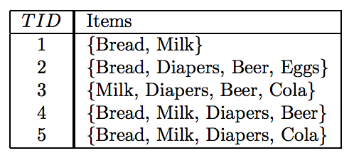
In the table above, each row is a unique transaction (usually identified by a unqiue id) and a set of items purchased within this transaction. These information can be useful for many business-related applications, but here we'll focus on a specific one called Association Analysis.

With Association Analysis, the outputs are association rules that explain the relationship (co-occurrence) between the items. A classic example is: {Beer} -> {Diapers}, which states that transactions including {Beer} tend to include {Diapers}. Or intuitively, it means that customer who buys beer also tends to buy diapers. With this information (If there is a pair of items, X and Y, that are frequently bought together), business can use them to:

Both X and Y can be placed on the same shelf, so that buyers of one item would be prompted to buy the other
Promotional discounts could be applied to just one out of the two items
Advertisements on X could be targeted at buyers who purchase Y
X and Y could be combined into a package

Besides using it in the business context to identify new opportunities for crossselling products to customers, association rules can also be used in other fields. In medical diagnosis for instance, understanding which symptoms tend to co-morbid can help improve patient care and medicine prescription or even pages visited on a website to understand the browsing patterns of people who came to your website. There's even an interesting story about strawberry pop tarts at the following link. Blog: Association Rule Mining – Not Your Typical Data Science Algorithm

Terminology¶

The next question is, how do we uncover these associations? Before we jump into that, let's look at some of the terminologies that we'll be using:

Itemset: A collection of k items is termed as an k-itemset. For instance, {Beer, Diapers, Milk} is an example of a 3-itemset. The null (or empty) set is an itemset that does not contain any items.

Association Rule: An association rule is an expression that takes the form $X \rightarrow Y$, where X and Y are disjoint itemsets, i.e. there is no common item between the two itemsets. Mathematically, $X \cap Y = \emptyset$. The hyperparamter support and confidence controls the rules that are generated.

Support Measures proportion of transactions in which an itemset appears. Consider the following table:

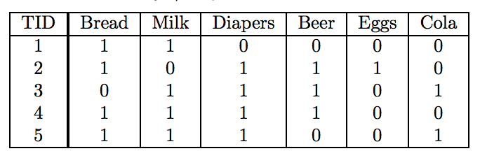
The table is just a binary representation of the first table above. Each row still corresponds to a transaction, but each column now corresponds to an item. Then the value in each cell is 1 if the item is present in a transaction and 0 otherwise.

For this table, the support count of {Milk, Diaper, Beer} is 2 and the support is 2 divided by the total number of transactions, which is 5. i.e. the support is 40%. Note that in these transactions if someone purchased two {Milk} in one transactions, the support will still remain the same, since we're only concerned about whether they purchased the item or not in the transaction.

Support is an important measure because a rule that has very low support may occur simply by chance. A low support rule is also likely to be uninteresting from a business perspective because it may not be profitable to promote items that customers seldom buy (unless it's something like diamond, house or a car).

Confidence measures how often the right hand side (RHS) item occurs in transactions containing the left-hand-side (LHS) item set. In other words, the confidence for the rule {X} -> {Y} can be computed by the formula: support count({X, Y}) / support count({X}). The interpretation for this step is saying how likely is item Y purchased when item X is purchased. e.g. in the table above, the confidence of {Milk} -> {Bread} is 3 out of 4, or 75%, because in the 4 transactions that contains the item {Bread}, there are 3 that contains both {Bread} and {Milk}.

Confidence measures the reliability of the inference made by a rule. For a given rule {X} -> {Y}, the higher the confidence, the more likely it is for Y to be present in transactions that contain X.

Apriori¶

A common strategy adopted by many association rule mining algorithms is to decompose the problem into two major subtasks:

Frequent Itemset Generation, whose objective is to find all the itemsets that satisfy the minimum support threshold. These itemsets are called frequent itemsets.
Rule Generation, whose objective is to extract all the high-confidence rules from the frequent itemsets found in the previous step.

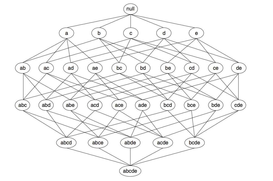
So starting with step 1, we wish to identify our frequent itemset. One possible way to do this is to list out every combination of items (the following diagram that shows all possible combination pairs for five items), obtain the corresponding count and see if it's greater than the support threshold that we've specified. This naive approach will definitely work, but a dataset that contains $N$ distinct items in total can generate $2^N - 1$ possible combinations. And doing this can be extremely slow!

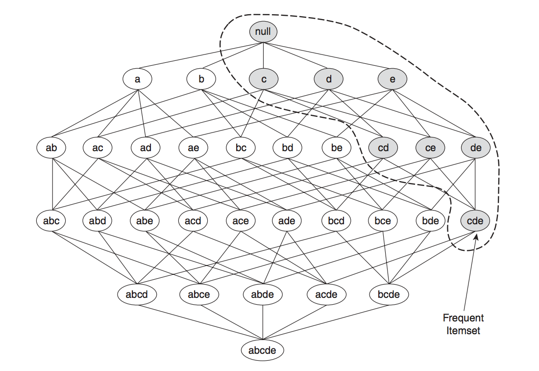
Now we'll start by looking at the widely known association analysis algorithm, Apriori. Apriori is based on the rule that if an itemset is infrequent, then all of its supersets are also infrequent. To see why this rule can be helpful, suppose we now know item {a} and {b} are already infrequent. Using the rule, we can automatically drop any supersets that contain {a} and {b}, because we know they will not surpass the minimum support threshold that we've set. In the diagram below, we can see that a large part of the diagram can be pruned (we now only need to compute the support for the grey node).

The figure below provides a high-level illustration of the frequent itemset generation part of the Apriori algorithm for the toy transactions data shown at the last section. We assume that the support threshold is 60% (this is a hyperparamter that we have to specify), which is equivalent to a minimum support count equal to 3.

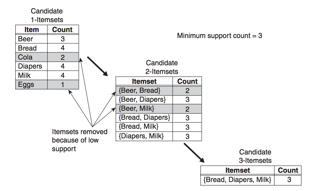
Initially, every item is considered as a candidate 1-itemset. After counting their supports, the candidate itemsets {Cola} and {Eggs} are discarded because they appear in fewer than 3 transactions. In the next iteration, candidate 2-itemsets are generated using only the frequent 1-itemsets. During the 2-itemsets stage, two of these six candidates, {Beer, Bread} and {Beer, Milk}, are subsequently found to be infrequent after computing their support values. The remaining four candidates are frequent, and thus will be used to generate the 3-itemsets candidate. The only candidate that has this property is {Bread, Diapers, Milk}.

Frequent Itemsets¶

def create_candidate_1(X):
    """
    create the 1-item candidate,
    it's basically creating a frozenset for each unique item
    and storing them in a list
    """
    c1 = []
    for transaction in X:
        for t in transaction:
            t = frozenset([t])
            if t not in c1:
                c1.append(t)
    return c1

def apriori(X, min_support):
    """
    pass in the transaction data and the minimum support 
    threshold to obtain the frequent itemset. Also
    store the support for each itemset, they will
    be used in the rule generation step
    """

    # the candidate sets for the 1-item is different,
    # create them independently from others
    c1 = create_candidate_1(X)
    freq_item, item_support_dict = create_freq_item(X, c1, min_support = 0.5)
    freq_items = [freq_item]
    
    k = 0
    while len(freq_items[k]) > 0:
        freq_item = freq_items[k]
        ck = create_candidate_k(freq_item, k)       
        freq_item, item_support = create_freq_item(X, ck, min_support = 0.5)
        freq_items.append(freq_item)
        item_support_dict.update(item_support)
        k += 1
        
    return freq_items, item_support_dict

def create_freq_item(X, ck, min_support):
    """
    filters the candidate with the specified
    minimum support
    """
    # loop through the transaction and compute
    # the count for each candidate (item)
    item_count = {}
    for transaction in X:
        for item in ck:
            if item.issubset(transaction):
                if item not in item_count: 
                    item_count[item] = 1
                else: 
                    item_count[item] += 1    
    
    n_row = X.shape[0]
    freq_item = []
    item_support = {}
    
    # if the support of an item is greater than the 
    # min_support, then it is considered as frequent
    for item in item_count:
        support = item_count[item] / n_row
        if support >= min_support:
            freq_item.append(item)
        
        item_support[item] = support
        
    return freq_item, item_support

def create_candidate_k(freq_item, k):
    """create the list of k-item candidate"""
    ck = []
    
    # for generating candidate of size two (2-itemset)
    if k == 0:
        for f1, f2 in combinations(freq_item, 2):
            item = f1 | f2 # union of two sets
            ck.append(item)
    else:    
        for f1, f2 in combinations(freq_item, 2):       
            # if the two (k+1)-item sets has
            # k common elements then they will be
            # unioned to be the (k+2)-item candidate
            intersection = f1 & f2
            if len(intersection) == k:
                item = f1 | f2
                if item not in ck:
                    ck.append(item)
    return ck

# X is the transaction table from above
# we won't be using the binary format
"""
X = np.array([[1, 1, 0, 0, 0, 0],
              [1, 0, 1, 1, 1, 0],
              [0, 1, 1, 1, 0, 1],
              [1, 1, 1, 1, 0, 0],
              [1, 1, 1, 0, 0, 1]])
"""
X = np.array([[0, 1],
              [0, 2, 3, 4],
              [1, 2, 3, 5],
              [0, 1, 2, 3],
              [0, 1, 2, 5]])
freq_items, item_support_dict = apriori(X, min_support = 0.5)
freq_items

[[frozenset({3}), frozenset({0}), frozenset({1}), frozenset({2})],
 [frozenset({2, 3}), frozenset({0, 2}), frozenset({1, 2}), frozenset({0, 1})],
 []]

Rules Generation¶

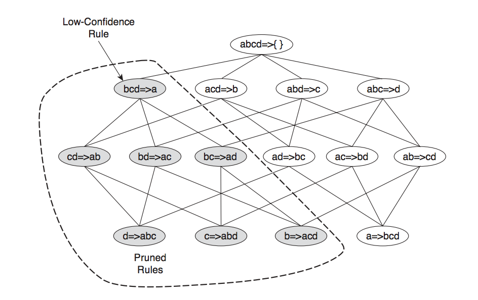
After creating our frequent itemsets, we proceed on to the rule generation stage. Apriori uses a level-wise approach for generating association rules, where each level corresponds to the number of items that belong to the rule's consequent (the rule's right hand side). Initially, the frequent itemset will create rules that have only one item in the consequent. These rules are then merged to create new candidate rules. For example, if we have a frequent itemset {abcd}, we will first create the rules {abc} -> {d} and {bcd} -> {a}, {acd} -> {b} and {abd} -> {c}. Then if only {acd} -> {b} and {abd} -> {c} are high-confidence rules, the candidate rule {ad} -> {bc} is generated by merging the consequents of both rules.

During this rule generating process, a useful rule is: if a rule $X \rightarrow Y − X$ does not satisfy the confidence threshold, then any rule $X' \rightarrow Y − X'$, where $X'$ is a subset of X, must not satisfy the confidence threshold as well. In the example below, we can see that: suppose the confidence for {bcd} -> {a} is low. All the rules containing item $a$ in its consequent, including {cd} -> {ab}, {bd} -> {ac}, {bc} -> {ad}, and {d} -> {abc} can be discarded.

Lift¶

Existing association rule mining algorithm relies on the support and confidence measures to eliminate uninteresting patterns. The drawback of support is that many potentially interesting patterns involving low support items might be eliminated by the support threshold. The drawback of confidence is more subtle and is best demonstrated with the following example.

Suppose we are interested in analyzing the relationship between people who drink tea and coffee. We may gather information about the beverage preferences among a group of people and summarize their responses into a table such as the one shown below:

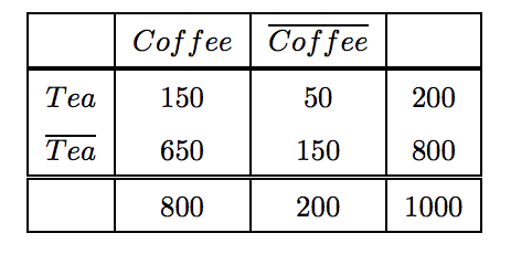
The information given in this table can be used to evaluate the association rule {Tea} -> {Coffee}. At first glance, it may appear that people who drink tea also tend to drink coffee because rule's support is 15% and the rule's confidence values is also reasonably high (75%, computed by 150 / 200). This argument would have been acceptable except that the fraction of people who drink coffee, regardless of whether they drink tea, is 80%, while the fraction of tea drinkers who drink coffee is only 75%. This points to a inverse relationship between tea drinkers and coffee drinkers.

To conclude the rule {Tea} -> {Coffee} can be misleading despite its high confidence value. The pitfall of the confidence masure is that it ignores the support of the itemset in the rule consequent. Due to the limitations in the support-confidence framework, various objective measures have been used to evaluate the quality of association patterns. The measure that we'll introduce is called Lift.

Lift. Suppose there's a rules {X} -> {Y}. The measure is the ratio between the rule’s confidence and the support of the itemset in the rule consequent. Or more formally: confidence ({X, Y}) / support ({Y}) ).

This says how likely item Y is purchased when item X is purchased, while controlling for how popular item Y is. A lift of 1 implies no association between items. A lift value greater than 1 means that item Y is likely to be bought if item X is bought (positively correlated), while a value less than 1 means that item Y is unlikely to be bought if item X is bought (negatively correlated).

def create_rules(freq_items, item_support_dict, min_confidence):
    """
    create the association rules, the rules will be a list.
    each element is a tuple of size 4, containing rules'
    left hand side, right hand side, confidence and lift
    """
    association_rules = []

    # for the list that stores the frequent items, loop through
    # the second element to the one before the last to generate the rules
    # because the last one will be an empty list. It's the stopping criteria
    # for the frequent itemset generating process and the first one are all
    # single element frequent itemset, which can't perform the set
    # operation X -> Y - X
    for idx, freq_item in enumerate(freq_items[1:(len(freq_items) - 1)]):
        for freq_set in freq_item:
            
            # start with creating rules for single item on
            # the right hand side
            subsets = [frozenset([item]) for item in freq_set]
            rules, right_hand_side = compute_conf(freq_items, item_support_dict, 
                                                  freq_set, subsets, min_confidence)
            association_rules.extend(rules)
            
            # starting from 3-itemset, loop through each length item
            # to create the rules, as for the while loop condition,
            # e.g. suppose you start with a 3-itemset {2, 3, 5} then the 
            # while loop condition will stop when the right hand side's
            # item is of length 2, e.g. [ {2, 3}, {3, 5} ], since this
            # will be merged into 3 itemset, making the left hand side
            # null when computing the confidence
            if idx != 0:
                k = 0
                while len(right_hand_side[0]) < len(freq_set) - 1:
                    ck = create_candidate_k(right_hand_side, k = k)
                    rules, right_hand_side = compute_conf(freq_items, item_support_dict,
                                                          freq_set, ck, min_confidence)
                    association_rules.extend(rules)
                    k += 1    
    
    return association_rules

def compute_conf(freq_items, item_support_dict, freq_set, subsets, min_confidence):
    """
    create the rules and returns the rules info and the rules's
    right hand side (used for generating the next round of rules) 
    if it surpasses the minimum confidence threshold
    """
    rules = []
    right_hand_side = []
    
    for rhs in subsets:
        # create the left hand side of the rule
        # and add the rules if it's greater than
        # the confidence threshold
        lhs = freq_set - rhs
        conf = item_support_dict[freq_set] / item_support_dict[lhs]
        if conf >= min_confidence:
            lift = conf / item_support_dict[rhs]
            rules_info = lhs, rhs, conf, lift
            rules.append(rules_info)
            right_hand_side.append(rhs)
            
    return rules, right_hand_side

association_rules = create_rules(freq_items, item_support_dict, min_confidence = 0.5)
association_rules

[(frozenset({3}), frozenset({2}), 1.0, 1.25),
 (frozenset({2}), frozenset({3}), 0.7499999999999999, 1.2499999999999998),
 (frozenset({2}), frozenset({0}), 0.7499999999999999, 0.9374999999999998),
 (frozenset({0}), frozenset({2}), 0.7499999999999999, 0.9374999999999998),
 (frozenset({2}), frozenset({1}), 0.7499999999999999, 0.9374999999999998),
 (frozenset({1}), frozenset({2}), 0.7499999999999999, 0.9374999999999998),
 (frozenset({1}), frozenset({0}), 0.7499999999999999, 0.9374999999999998),
 (frozenset({0}), frozenset({1}), 0.7499999999999999, 0.9374999999999998)]

Table of Contents